Anticipative kinodynamic planning:multi-objective robot navigation in urban and dynamic environments [Social Force.pdf](C:\Users\adminnus\OneDrive - National University of Singapore\B_Reading Materials\A_Path Planning\Papers\Prediction\Social Force.pdf)
Behavior estimation for a complete framework for human motion prediction in crowded environments [Social Force 2.pdf](C:\Users\adminnus\OneDrive - National University of Singapore\B_Reading Materials\A_Path Planning\Papers\Prediction\Social Force 2.pdf)
Probabilistic Methods
Probabilistic Trajectory Prediction with Gaussian Mixture Models, Intelligent Vehicles Symposium, 2012. [Probabilistic Trajectory Prediction with Gaussian Mixture Models.pdf](C:\Users\adminnus\OneDrive - National University of Singapore\B_Reading Materials\A_Path Planning\Papers\Prediction\Probabilistic Trajectory Prediction with Gaussian Mixture Models.pdf).
GMM: point estimate for model parameter
Solving method: iterative EM
infer joint Gaussian mixture distribution $p(\mathbb x_f, \mathbb x_h)$, then predict by using conditional mixture density $p(\mathbb x_f | \mathbb x_h)$
VGMM: prior distribution over parameters, then derive full Bayesian treatment.
Not point estimate, parameters are given conjugate prior distribution.
Solving method: Variational Bayesian EMs
similarly, infer joint distribution, then obtian conditional distribution.
Compare Two Methods.
How Would Surround Vehicles Move? A Unified Framework for Maneuver Classification and Motion Prediction, IEEE Transactions on Intelligent Vehicles, 2018. [How Would Surround Vehicles Move_A Unified Framework for Maneuver Classification and Motion Prediction.pdf](C:\Users\adminnus\OneDrive - National University of Singapore\B_Reading Materials\A_Path Planning\Papers\Prediction\How Would Surround Vehicles Move_A Unified Framework for Maneuver Classification and Motion Prediction.pdf)
Vehicle Speed Prediction Using a Markov Chain With Speed Constraints, IEEE Transactions on ITS. 2018. [Vehicle Speed Prediction Using a Markov Chain With Speed Constraints.pdf](C:\Users\adminnus\OneDrive - National University of Singapore\B_Reading Materials\A_Path Planning\Papers\Prediction\Vehicle Speed Prediction Using a Markov Chain With Speed Constraints.pdf)
Probabilistic Trajectory Prediction with Gaussian Mixture Models
Trajectory Representation
input data: short trajectory pieces.
Trajectory $T$: $$ T = ((x_0,y_0,z_0),t0), \cdots, ((x_{N-1},y_{N-1},z_{N-1}),t_{N-1}) described by $p_X, p_y, p_z$ $$ described by $p_X, p_y, p_z$ or described by roll, pitch and yaw angle $\phi(t_i), \theta(t_i), \psi(t_i)$ and velocity $v_x, v_y,v_z$.
Chebyshev decomposition on the components of trajectory $\rightarrow$ coefficients as input features of GMM
To approximate any arbitrary function $f(x)$ in $[-1,1]$, the Chebyshev coefficients are $$ c_n = \frac {2}{N} \sum\limits_{k=0}^{N-1} f(x_k) T_n(x_k) $$ where $x_k$ are N zeros of $T_N(x)$.
reformulate as $$ f(x) \approx \sum\limits_{n=0}^{m-1} c_n T_n(x) -\frac{1}{2}c_0 $$
This differs from our discussion of EM only in that the parameter vector $\theta$ no longer appears, because the parameters are now stochastic variables and are absorbed into $\mathbf Z$.
maximize the lower bound $\mathcal L$ = minimize the KL divergence.
In particular, there is no ‘over-fitting’ associated with highly flexible distributions. Using more flexible approximations simply allows us to approach the true posterior distribution more closely.
One way to restrict the family of approximating distributions is to use a parametric distribution $q(Z|ω)$ governed by a set of parameters $ω$. The lower bound $\mathcal L(q)$ then becomes a function of $ω$, and we can exploit standard nonlinear optimization techniques to determine the optimal values for the parameters.
Method:
Factorized distribution approximate to true posterior distribution –>> Mean field theory $$ KL(p||q) \quad \iff \quad KL(q||p) $$
if we consider approximating a multimodal distribution by a unimodal one,
Both types of multimodality were encountered in Gaussian mixtures, where they manifested themselves as multiple maxima in the likelihood function, and a variational treatment based on the minimization of $KL(q||p)$ will tend to find one of these modes.
if we were to minimize $KL(p||q)$, the resulting approximations would average across all of the modes and, in the context of the mixture model, would lead to poor predictive distributions (because the average of two good parameter values is typically itself not a good parameter value). It is possible to make use of $KL(p||q)$ to define a useful inference procedure, but this requires a rather different approach about expectation propagation.
The two forms of KL divergence are members of the alpha family of divergence.
Variational Mixture of Gaussian
Likelihood function $p(\mathbf Z| \mathbf \pi) = \prod\limits_{n=1}^N \prod\limits_{k=1}^K \pi_k^{z_{nk}}$
Conditional distribution of observed data $p(\mathbf X|\mathbf Z,\mu, \Lambda) = \prod\limits_{n=1}^N \prod\limits_{k=1}^K \mathcal N(\mathbf x_n|\mu_k,\Lambda_k^{-1})^{z_{nk}}$
Variables such as $\mathbb z_n$ that appear inside the plate are regarded as latent variables because the number of such variables grows with the size of the data set. By contrast, variables such as μ that are outside the plate are fixed in number independently of the size of the data set, and so are regarded as parameters
This effect can be understood qualitatively in terms of the automatic trade-off in a Bayesian model between fitting the data and the complexity of the model, in which the complexity penalty arises from components whose parameters are pushed away from their prior values.
Thus the optimization of the variational posterior distribution involves cycling between two stages analogous to the E and M steps of the maximum likelihood EM algorithm.
Variational E-step
use the current distributions over the model parameters to evaluate the moments in (10.64), (10.65), and (10.66) and hence evaluate $\mathbb E[z_{nk}] = r_{nk}$.
Variational M-step
keep these responsibilities fixed and use them to re-compute the variational distribution over the parameters using (10.57) and (10.59). In each case, we see that the variational posterior distribution has the same functional form as the corresponding factor in the joint distribution (10.41). This is a general result and is a consequence of the choice of conjugate distributions.
==variational EM v.s. EM for maximum likelihood.==
In fact if we consider the limit $N\rightarrow \infty$ then the Bayesian treatment converges to the maximum likelihood EM algorithm.
For anything other than very small data sets, the dominant computational cost of the variational algorithm for Gaussian mixturesa rises from the evaluation of the responsibilities, together with the evaluation and inversion of the weighted data covariance matrices. These computations mirror precisely those that arise in the maximum likelihood EM algorithm, and so there is little computational overhead in using this Bayesian approach as compared to the traditional maximum likelihood one.
The singularities that arise in maximum likelihood when a Gaussian component ‘collapses’ onto a specific data point are absent in the Bayesian treatment. Indeed, these singularities are removed if we simply introduce a prior and then use a MAP estimate instead of maximum likelihood.
Furthermore, there is no over-fitting if we choose a large number $K$ of components in the mixture.
Finally, the variational treatment opens up the possibility of determining the optimal number of components in the mixture without resorting to techniques such as cross validation.
Variational lower bound
Function:
to monitor the bound during the re-estimation in order to test for convergence
provide a valuable check on both the mathematical expressions for the solutions and their software implementation, because at each step of the iterative re-estimation procedure the value of this bound should not decrease.
provide a deeper test of the correctness of both the mathematical derivation of the update equations and of their software implementation by using finite differences to check that each update does indeed give a (constrained) maximum of the bound
lower bound provides an alternative approach for deriving the variational re-estimation equations in variational EM. To do this we use the fact that, since the model has conjugate priors, the functional form of the factors in the variational posterior distribution is known, namely discrete for $\mathbf Z$, Dirichlet for $π$, and Gaussian-Wishart for $(μ_k,Λ_k)$. By taking general parametric forms for these distributions we can derive the form of the lower bound as a function of the parameters of the distributions. Maximizing the bound with respect to these parameters then gives the required re-estimation equations.
Predictive density
predictive density for a new value $\hat x$ of the observed variable. corresponding to latent variable $\hat{\mathbf z}$. $$ p(\widehat{\mathbf{x}} | \mathbf{X})=\sum_{\widehat{\mathbf{z}}} \iiint p(\widehat{\mathbf{x}} | \widehat{\mathbf{z}}, \mu, \Lambda) p(\widehat{\mathbf{z}} | \boldsymbol{\pi}) p(\boldsymbol{\pi}, \boldsymbol{\mu}, \boldsymbol{\Lambda} | \mathbf{X}) \mathrm{d} \boldsymbol{\pi} \mathrm{d} \boldsymbol{\mu} \mathrm{d} \boldsymbol{\Lambda} \ = \sum_{k=1}^K \iiint \pi_k \mathcal N(\hat{\mathbf x} |\mu_k,\Lambda_k) q(\pi) q(\mu_k, \Lambda_k) d\pi d\mu_k d \Lambda_k $$ remaining integrations can now be evaluated analytically giving a mixture of Student’s t-distributions: $$ \begin{aligned} p(\widehat{\mathbf{x}} | \mathbf{X})&= \frac{1}{\widehat{\alpha}} \sum_{k=1}^{K} \alpha_{k} \operatorname{St}\left(\widehat{\mathbf{x}} | \mathbf{m}{k}, \mathbf{L}{k}, \nu_{k}+1-D\right) \ \qquad \mathbf{L}{k}&=\frac{\left(\nu{k}+1-D\right) \beta_{k}}{\left(1+\beta_{k}\right)} \mathbf{W}_{k} \end{aligned} $$ where $\mathbf m_k$ is the mean of $k$th component.
Determining the number of components.
variational lower bound can be used to determine a posterior distribution over the number $K$ of components in the mixture model.
If we have a mixture model comprising $K$ components, then each parameter setting will be a member of a family of $K!$ equivalent settings.
in EM, this is irrelevant because the parameter optimization algorithm will, depending on the initialization of the parameters, find one specific solution, and the other equivalent solutions play no role.
in Variational EM, we marginalize over all possible parameter values.
if the true posterior distribution is multimodal, variational inference based on the minimization of $KL(q||p)$ will tend to approximate the distribution in the neighborhood of one of the modes and ignore the others.
If we want to compare different value of $K$, we need to consider the multimodality.
Solution:
to add a term $\ln K!$ onto the lower bound when used for model comparison and averaging.
treat the mixing coefficients $π$ as parameters and make point estimates of their values by maximizing the lower bound with respect to $π$ instead of maintaining a probability distribution over them as in the fully Bayesian approach.
This leads to the re-estimation equation and this maximization is interleaved with the variational updates for the $q$ distribution over the remaining parameters.
Components that provide insufficient contribution to explaining the data will have their mixing coefficients driven to zero during the optimization, and so they are effectively removed from the model through automatic relevance determination. This allows us to make a single training run in which we start with a relatively large initial value of K, and allow surplus components to be pruned out of the model.
==Comparison:==
maximum likelihood would lead to values of the likelihood function that increase monotonically with K (assuming the singular solutions have been avoided, and discounting the effects of local maxima) and so cannot be used to determine an appropriate model complexity.
By contrast, Bayesian inference automatically makes the trade-off between model complexity and fitting the data.
based on input data to compute a distribution $P(x)$.
Idea: Use Gaussian distribution can function as approximate distribution to simulate the real distribution
<用已知的分布模拟未知的分布>
Parameters:
input: $x$
hidden variable: $z$
is parameter in real distribution. For GMM, $z$ is the mean and covariance of all gaussian distribution.
Posterior distribution $P(z|x)$:
using the data to guess the model. <用输入去推断隐含变量>
likelihood distribution $P(x|z)$:
distribution based on the model parameter.
distribution of input $P(x)$
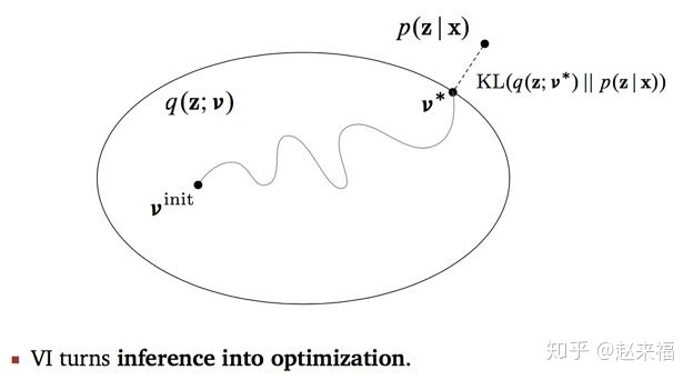
Prior distribution $q(z,v)$:
the distribution to simulate the real distribution. $z$ is hidden variables, $v$ is the parameter of distribution about $z$, i.e., hyperparameter.
normally, the distribution about $z$ is conjugate distribution.
Task:
adjust $v$ to make the approximate distribution close to the posterior distribution $p(z|x)$
Hope the posterior distribution and the prior distribution closed to 0. But the posterior distribution is unknown. Therefore, introduce the KL divergence and ELBO. $$ \log p(x) = KL(q(z;v) || p(z|x)) + ELBO(v) $$ because $\log p(x)$ is constant, the minimum KL divergence is the maximum ELBO.
Conv2D(filters, kernel_size, strides, padding, activation=None, use_bias=True) # "padding='valid'" means there is no padding, "padding='same'" means output dim is the same as input dim.
Here, nn.relu() has an argument inplace, which means the operation will be in-place. In other words, inplace=True means that it will modify the input directly, without allocating any additional output. It can sometimes slightly decrease the memory usage, but may not always be a valid operation (because the original input is destroyed)。利用in-place计算可以节省内(显)存,同时还可以省去反复申请和释放内存的时间。但是会对原变量覆盖,只要不带来错误就用。
lincon Constrained linear quadratic controller for linear systems
L=lincon(SYS,TYPE,COST,INTERVAL,LIMITS,QPSOLVER) build a regulator (or a controller for reference tracking) based on a finite time linear quadratic constrained optimal control formulation
SYS is the discrete-time linear time-invariant model (A,B,C,D,TS)
x(t+1) = Ax(t) + B [u(t-1)+du(t)] %du(t) = u(t)-u(t-1) = input increment y(t) = Cx(t) + D [u(t-1)+du(t)]
COST is a structure of weights with fields:
1 2 3 4 5 6 7
.Q = weight Q on states [ x'(k)Qx(k) ] (regulator only) .R = weight R on inputs [ u'(k)Ru(k) ] (regulator only) .P = weight P on final state [ x'(N)Px(N) ] (regulator only) .S = weight S on outputs [ (y(k)-r)'S(y(k)-r) ] (tracking only) .T = weight T on input increments [ du'(k) T du(k) ] (tracking only) .rho = weight on slack var [ rho*eps^2 ] (regulator and tracking) %rho=Inf means hard output constraints .K = feedback gain (default: K=0) [ u(k)=K*x(k) for k>=Nu] (only regulator)
Only for regulators: If COST.P='lqr' then P is chosen as the solution of the LQR problem with weights Q,R, and K is chosen as the corresponding LQR gain. If COST.P='lyap' then P is chosen as the solution of the Lyapunov equation A'PA - P + Q = 0, and K=0 (default).
INTERVAL is a structure of number of input and output optimal control steps
1 2 3 4
.N = optimal control interval over which the cost functionissummed .Nu = number of free optimal control moves u(0),...,u(Nu-1) .Ncy = output constraints are checked up to time k=Ncy .Ncu = input constraints are checked up to time k=Ncu
LIMITS is a structure of constraints with fields:
1 2 3 4 5 6
.umin = lower bounds on inputs [ u(k)>=umin ] .umax = upper bounds on inputs [ u(k)<=umax ] .ymin = lower bounds on outputs [ y(k)>=ymin ] .ymax = upper bounds on outputs [ y(k)<=ymax ] .dumin = lower bounds on input increments [ du(k)>=dumin ] (only tracking) .dumax = upper bounds on input increments [ du(k)<=dumax ] (only tracking)
Only for regulators:* If COST.P='lqr' then P is chosen as the solution of the LQR problem with weights Q,R, and K is chosen as the corresponding LQR gain. If COST.P='lyap' then P is chosen as the solution of the Lyapunov equation A'PA - P + Q = 0, and K=0 (default).
QPSOLVER specifies the QP used for evaluating the control law. Valid options are:
1 2 3 4 5
'qpact' active set method 'quadprog' QUADPROG from Optimization Toolbox 'qp' QP from Optimization Toolbox 'nag' QP from NAG Foundation Toolbox 'cplex' QP from Ilog Cplex
YZEROCON enforce output constraints also at prediction time k=0 if YZEROCON=1 (default: YZEROCON=0).
If YEZEROCON is a 0/1 vector of the same dimension as the output vector, then only those outputs where YZEROCON(i)=1 are constrained at time k=0.
Time-varying formulation: Use the same syntax as above, with input arguments as follow:
SYS = cell array of linear models, SYS{i}=model used to predict at step t+i-1
COST = cell array of structures of weights: COST{i}.Q, COST{i}.R, etc. Only COST{1}.rho is used for penalty soft constraint penalty, COST{i}.rho is ignored for i>1.
LIMITS = cell arrays of structures of upper and lower bounds: LIMITS{i}.umin, etc. The constraints LIMITS{i} refer to time index t+i, for both inputs and outputs.linsfun
sim for lincon
sim : Closed-loop simulation of constrained optimal controllers for linear systems.
[X,U,T,Y]=sim(LINCON,MODEL,refs,x0,Tstop,u0,qpsolver,verbose) simulates the closed-loop of the linear system MODEL with the controller LINCON based on quadratic programming.
Usually, LINCON is based on model MODEL (nominal closed-loop).
1 2 3 4 5 6 7 8 9
Input:
LINCON = optimal controller refs = structure or references with fields; ref.y output references (only for tracking) x0 = initial state Tstop = total simulation time (total number of steps = Tstop/LINCON.Ts) u0 = input at time t=-1 (only for tracking) qpsolver = QP solver (type HELP QPSOL for details) verbose = verbosity level (0,1)
refs.y has as many columns as the number of outputs
1 2 3 4 5 6
Output arguments: X is the sequence of states, with as many columns as the number of states. U is the sequence of inputs, with as many columns as the number of inputs. T is the vector of time steps. I is the sequence of region numbers Y is the sequence of outputs, with as many columns as the number of outputs.
Without output arguments, sim produces a plot of the trajectories
LINCON objects based on time-varying prediction models/weights/limits can be simulated in closed-loop with LTI models. Time-varying simulation models are not supported, use custom for-loops instead.
sim (general)
sim : Simulate a Simulink model
SimOut = sim('MODEL', PARAMETERS) simulates your Simulink model,
'PARAMETERS' represents a list of parameter name-value pairs, a structure containing parameter settings, or a configuration set.
SimOut returned by the sim command is an object that contains all of the logged simulation results.
PARAMETERS can be used to override existing block diagram configuration parameters for the duration of the simulation.
1 2 3 4 5 6 7 8
This syntax is referred to as the 'Single-Output Format'. paramNameValStruct.SimulationMode = 'rapid'; paramNameValStruct.AbsTol = '1e-5'; paramNameValStruct.SaveState = 'on'; paramNameValStruct.StateSaveName = 'xoutNew'; paramNameValStruct.SaveOutput = 'on'; paramNameValStruct.OutputSaveName = 'youtNew'; simOut = sim('vdp',paramNameValStruct)
kalman
KALMANDesign Kalman filter for constrained optimal controllers
KALMAN(CON,Q,R) design a state observer for the linear model (A,B,C,D)=CON.model which controller CON is based on, using Kalman filtering techniques. The resulting observer is stored in the 'Observer' field of the controller object. The controller object can be either of class LINCON or EXPCON.
Q is the covariance matrix of state noise, R is the covariance matrix of outputnoise.
Kest=KALMAN(CON,Q,R) also return the state observer as an LTI object.
Kest receives u[n] and y[n] as inputs (in this order), and provides the best estimated state x[n|n-1] of x[n] given the past measurements y[n-1], y[n-2],...
Kest=KALMAN(CON,Q,R,ymeasured) assumes that only the outputs specified in vector ymeasured are measurable outputs. In this case, R is a nym-by-nym matrix, where nym is the number of measured outputs.
[Kest,M]=KALMAN(CON,Q,R,ymeasured) also returns the gain M which allows computing the measurement update
1
x[n|n] = x[n|n-1] + M(y[n] - Cx[n|n-1] - Du[n])
For time-varying prediction models, the first model CON.model{1} is used to build the Kalman filter, as it is the model of the process for the current time step.
**E=EXPCON(C,RANGE,OPTIONS) **convert controller C to piecewise affine explicit form.
C is a constrained optimal controller for linear systems or hybrid systems (an object of class @LINCON or @HYBCON)
RANGE defines the range of the parameters the explicit solution is found with respect to (it may be different from the limits over variables imposed in the control law). RANGE is a structure with fields:
1 2 3 4 5
.xmin, xmax = range of states [ xmin <= x <= xmax ] (linear and hybrid) .umin, umax = range of inputs [ umin <= u <= umax ] (linear w/ tracking) .refymin, refymax = range of output refs [ refymin <= r.y <= refymax] (linear w/ tracking and hybrid) .refxmin, refxmax = range of state refs [ refxmin <= r.x <= refxmax ] (hybrid) .refumin, refumax = range of input refs [ refumin <= r.u <= refumax ] (hybrid)
For hybrid controllers, refxmin,refxmax,refumin,refumax,refymin,refymax must have dimensions consistent with the number of indices specified in C.ref (type “help hybcon” for details)
OPTIONS defines various options for computing the explicit control law:
1 2 3 4 5 6 7 8 9 10 11 12
.lpsolver = LP solver (type HELP LPSOL for details) .qpsolver = QP solver (type HELP QPSOL for details) .fixref = structure with fields 'y','x','u' defining references that are fixed at given values, therefore simplifying the parametric solution [hybrid only] .valueref = structure with fields 'y','x','u' of values at which references are fixed [hybrid only] .flattol Tolerance for a polyhedral set to be considered flat .waitbar display waitbar (only for hybrid) .verbose = level of verbosity {0,1,2} of mp-PWA solver .mplpverbose = level of verbosity {0,1,2} of mp-LP solver .uniteeps = tolerance for judging convexity of the union of polyhedra .join = flag for reducing the complexity by joining regions whose union is a convex set. .reltol = tolerance used for several polyhedral operations .sequence = flag for keeping the entire optimal control sequence as an explicit functionoftheparametersalsointhelinearcase. Flagignoredinthehybridcase: sequencealwaysstoredwithquadraticcosts, neverstoredwithinf-norms.
Example: to fix the reference signal for x(1),x(2) at the values rx(1)=0.6, rx(2)=-1.4 and mantain the reference rx(3) for x(3) as a free parameter, specify options.fixref.x=[1 2], options.valueref.x=[0.6 -1.4].
Note: @MPC objects from MPC Toolbox are no longer supported, as they are handled directly in the MPC Toolbox since R2014b.
See also EXPCON/EVAL for the order states and references are stored inside the parameter vector.
##Modelling
tf
Create transfer function model; 2. convert to transfer function model
sys = ss(A,B,C,D) creates a state-space model object representing the continuous-time state-space model
$x=Ax+Bu$
$y=Cx+Du$
For a model with Nx states, Ny outputs, and Nu inputs:
- A is an Nx-by-Nx real- or complex-valued matrix.
- B is an Nx-by-Nu real- or complex-valued matrix.
C is an Ny-by-Nx real- or complex-valued matrix.
D is an Ny-by-Nu real- or complex-valued matrix.
To set D = 0 , set D to the scalar 0 (zero), regardless of the dimension.
sys = ss(A,B,C,D,Ts) creates the discrete-time model
$x[n+1]=Ax[n]+Bu[n]$
$y[n]=Cx[n]+Du[n]$
with sample time Ts (in seconds). Set Ts = -1 or Ts = [] to leave the sample time unspecified.
ssdata
ssdata : Quick access to state-space data.
[A,B,C,D] = ssdata(SYS) returns the A,B,C,D matrices of the state-space model SYS. If SYS is not a state-space model, it is first converted to the state-space representation. If SYS is in descriptor form (nonempty E matrix), an equivalent explicit form is first derived. If SYS has internal delays, A,B,C,D are obtained by first setting all internal delays to zero (delay-free dynamics).
[A,B,C,D,TS] = ssdata(SYS) also returns the sample time TS. Other properties of SYS can be accessed using struct-like dot syntax (for example, SYS.StateName).
Support for arrays of state-space models:
[A,B,C,D,TS] = ssdata(SYS,J1,...,JN) extracts the data for the (J1,…,JN) entry in the model array SYS.
If all models in SYS have the same order, ssdata returns multi-dimensional arrays A,B,C,D where A(:,:,k), B(:,:,k), C(:,:,k), D(:,:,k) are the state-space matrices of the k-th model SYS(:,:,k).
If the models in SYS have variable order, use the syntax [A,B,C,D] = ssdata(SYS,'cell') to extract the state-space matrices of each model as separate cells in the cell arrays A,B,C,D.
[X,L,G] = dare(A,B,Q,R,S,E) computes the unique stabilizing solution X of the discrete-time algebraic Riccati equation $E’XE = A’XA - (A’XB + S)(B’XB + R)^{-1} (A’XB + S)’ + Q$ or, equivalently (if R is nonsingular) $E’XE = F’XF - F’XB(B’XB + R)^{-1} B’XF + Q - SR^{-1} S’$ with $F:=A-BR^{-1}S’$.
When omitted, $R$, $S$ and $E$ are set to the default values $R=I$ , $S=0$ , and $E=I$. Beside the solution X, dare also returns the gain matrix $G = (B’XB + R)^{-1}(B’XA + S’)$, and the vector $L$ of closed-loop eigenvalues (i.e., EIG(A-B*G,E)).
[X,L,G,REPORT] = dare(...) returns a diagnosis REPORT with value:
-1 if the Symplectic matrix has eigenvalues on the unit circle
-2 if there is no finite stabilizing solution X
Frobenius norm of relative residual if X exists and is finite. This syntax does not issue any error message when X fails to exist.
[X1,X2,D,L] = dare(A,B,Q,...,'factor') returns two matrices X1, X2 and a diagonal scaling matrix D such that $X = D(X_2/X_1)D$. The vector $L$ contains the closed-loop eigenvalues. All outputs are empty when the associated Symplectic matrix has eigenvalues on the unit circle
dlqr
dlqr : Linear-quadratic regulator design for discrete-time systems.
[K,S,E] = dlqr(A,B,Q,R,N) calculates the optimal gain matrix $K$ such that the state-feedback law u[n] = -Kx[n] minimizes the cost function
J = Sum {x'Qx + u'Ru + 2*x'Nu}
subject to the state dynamics x[n+1] = Ax[n] + Bu[n].
The matrix N is set to zero when omitted. Also returned are the Riccati equation solution S and the closed-loop eigenvalues E :
1
A'SA - S - (A'SB+N) (R+B'SB)^(-1) (B'SA+N') + Q = 0, E = EIG(A-B*K)
lqr
lqr : Linear-quadratic regulator design for state space systems.
[K,S,E] = lqr(SYS,Q,R,N) calculates the optimal gain matrix K such that:
For a continuous-time state-space model SYS, the state-feedback law u = -Kx minimizes the cost function
1
J = Integral {x'Qx + u'Ru + 2*x'Nu} dt
subject to the system dynamics dx/dt = Ax + Bu
For a discrete-time state-space model SYS, u[n] = -Kx[n] minimizes
1
J = Sum {x'Qx + u'Ru + 2*x'Nu}
subject to x[n+1] = Ax[n] + Bu[n].
The matrix N is set to zero when omitted. Also returned are the solution S of the associated algebraic Riccati equation and the closed-loop eigenvalues E = EIG(A-B*K) .
[K,S,E] = lqr(A,B,Q,R,N) is an equivalent syntax for continuous-time models with dynamics dx/dt = Ax + Bu
operspec
operspec : Create operating point specifications for Simulink model.
OP = operspec('sys') returns an operating point specification object OP, for a Simulink model 'sys'. Edit the default operating point specifications directly or use get and set. Use the operating point specifications object with the function FINDOP to find operating points based on the specifications. Use these operating points with the function LINEARIZE to create linearized models.
OP = operspec('sys', N) returns an N-dimensional column vector of the default operating point specification objects for a Simulink model 'sys'.
OP = operspec('sys', SIZE) returns an array of the default operating point specification objects. The size of OP is specified in the SIZE vector. For example, operspec('vdp', [2,3]) returns a 2-by-3 matrix of default operating point specifications for the Simulink model 'vdp'.
findop
findop : Find operating points from specifications or simulation
place
place Pole placement design
1 2
K = place(A,B,p) [K,prec,message] = place(A,B,p)
Given the single- or multi-input system $x=Ax+Bu$, and a vector p of desired self-conjugate closed-loop pole locations, place computes a gain matrix K such that the state feedback u=-Kx places the closed-loop poles at the locations p. In other words, the eigenvalues of A – BK match the entries of p (up to the ordering).
K = place(A,B,p) places the desired closed-loop poles p by computing a state-feedback gain matrix K. All the inputs of the plant are assumed to be control inputs. The length of p must match the row size of A. place works for multi-input systems and is based on the algorithm from [1]. This algorithm uses the extra degrees of freedom to find a solution that minimizes the sensitivity of the closed-loop poles to perturbations in A or B.
[K,prec,message] = place(A,B,p) returns prec, an estimate of how closely the eigenvalues of A – BK match the specified locations p (prec measures the number of accurate decimal digits in the actual closed-loop poles). If some nonzero closed-loop pole is more than 10% off from the desired location, message contains a warning message.
mpc
mpc Create an mpc controller.
MPCOBJ = mpc(PLANT) creates the mpc object based on the linear plant model PLANT, which must be a SS, TF, ZPK or a linear model from System Identification Toolbox such as IDSS, IDTF, IDPROC, IDPOLY and IDGREY.
MPCOBJ = mpc(PLANT,TS) specifies a sampling time for the mpc controller. A continuous-time PLANT model is discretized with sampling time TS. A discrete-timePLANT model is resampled to sampling time TS.
MPCOBJ = mpc(PLANT,TS,P) specifies the prediction horizon P. P is a positive, finite integer.
MPCOBJ = mpc(PLANT,TS,P,M) specifies the control horizon M. M is either an integer (<= P) or a vector of blocked moves such that sum(M)<= P.
MPCOBJ = mpc(PLANT,TS,P,M,Weights,MV,OV,DV) also allows you to specify Weights, constraints on MV, MV rates and plant outputs, scale factors, as well as other properties with structures Weights, MV, OV and DV in that order. Those properties can also be specified using either
1
SET(MPCOBJ,Property1,Value1,Property2,Value2,...)
or
1
MPCOBJ.Property = Value
Disturbance models and operating conditions can be specified using the syntax:
1 2 3 4 5 6 7
MPCOBJ = mpc(MODELS,TS,P,M) where MODELS is a structure containing MODELS.Plant = plant model (LTI or linear model from System Identification Toolbox). .Disturbance = model describing the input disturbances. This model is assumed to be driven by unit variance white noise. .Noise = model describing the plant output measurement noise. This model is assumed to be driven by unit variance white noise. .Nominal = structure specifying the plant nominal conditions at which the plant was linearized. MPCOBJ = mpc creates an empty mpc object
initial
initial Initial condition response of state-space models.
initial(SYS,X0) plots the undriven response of the state-space model SYS (created with SS) with initial condition X0 on the states. This response is characterized by the equations . Continuous time: $ x = A x ,\ y = C x ,\ x(0) = x_0 $
The time range and number of points are chosen automatically.
initial(SYS,X0,T) uses the time vector T for simulation (expressed in the time units of SYS). For discrete-time models, T should be of the form Ti:Ts:Tf where Ts is the sample time. For continuous-time models, T should be of the form Ti:dt:Tf where dt is the sampling period for the discrete approximation of SYS.
initial(SYS,X0,T) uses the time vector T for simulation (expressed in the time units of SYS). For discrete-time models, T should be of the form Ti:Ts:Tf where Ts is the sample time. For continuous-time models, T should be of the form Ti:dt:Tf where dt is the sampling period for the discrete approximation of SYS.
run sim
lsim
lsim Simulate time response of dynamic systems to arbitrary inputs.
lsim(SYS,U,T) plots the time response of the dynamic system SYS to the input signal described by U and T. The time vector T is expressed in the time units of SYS and consists of regularly spaced time samples. The matrix U has as many columns as inputs in SYS and its i-th row specifies the input value at time T(i). For example, t = 0:0.01:5; u = sin(t); lsim(sys,u,t) simulates the response of a single-input model SYS to the input u(t)=sin(t) during 5 time units.
For discrete-time models, U should be sampled at the same rate as SYS (T is then redundant and can be omitted or set to the empty matrix). For continuous-time models, choose the sampling period T(2)-T(1) small enough to accurately describe the input U. lsim issues a warning when U is undersampled and hidden oscillations may occur.
msgbox
msgbox : Create message dialog box
1
2
3
4
5
f = msgbox(message) f = msgbox(message,title) f = msgbox(message,title,icon) f = msgbox(message,title,'custom',icondata,iconcmap) f = msgbox(___,createmode)
warndlg
Create warning dialog box
1 2 3 4
f = warndlg(msg)
f = warndlg(msg,title)
f = warndlg(msg,title,opts)
f = warndlg
waitfor
waitfor : Block execution and wait for condition [after operation, will terminate the message box]
Chance-Constrained Optimal Path Planning with Obstacles
Prior works: Set-Bound Uncertainty
Key idea: use bounds on the probability of collision to approximate the nonconvex chance-constrained optimization problem as a disjunctive convex problem. Then, solve by Branch-and-Bound techniques.
Target: linearm discrete-time system.
UAV. Uncertainty:
location is not exactly known, but is estimated using a system model, interior sensors, and/or global position system. distribution may be generated with estimation technique, like KF.
$\rightarrow$ initial position is Gaussian distribution.
system model are approximations of true system model and these dynamixss are not fully known.
$\rightarrow$ model uncertainty to be Gaussian white noise
disturbances makes the turue trajecotyr. deviate from the palnned trajectory.
$\rightarrow$ modeled as Gaussian noise on dynamics.
Prior Method: Set-bounded uncertainty models. to make sure the disturbance do not exceed the bounds.
Chance Constraints:
Advantages over set-bounded approach:
disturbances are represented using a stochastic model, rather than set-bounded one.
When use KF as localization, state estimate is a probabilsitic function with mean and covariancel
Existing CCP of linear system s.t. Gaussian uncertainty in convex region.
This paper extend to nonconvex region.
Key: bound the probability of collision, give conservative approximation, formulate as disjunctive convex program, solve by Branch-and-Bound techniques.
Convex region:
Nonconvex region:
Early, convert problem into set-bound by ensuring 3-$\sigma$ confidence region. Then, can solve. But fail to ding a feasible solution.
Particle-based approach. Approximate the chance constraint, but not guarantee satisfaction of constraint. Can use arbitrary uncertainty distribution, rather than only Gaussian. But Computational intensive.
Anylytic bound to ensure the satifaction of constraints. little conservatism.
$\omega_t$ is Gaussian white noise with $\omega_t \sim \mathcal{N}(0,Q)$
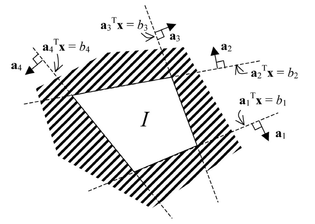
polygonal convex stay-in regions $\mathcal{I}$: states much remain $$ \mathcal{I} \Longleftrightarrow \bigwedge_{t \in T(\mathcal{I})} \bigwedge_{i \in G(\mathcal{I})} \mathbf{a}{i}^{\prime} \mathbf{x}{t} \leq b_{i} $$
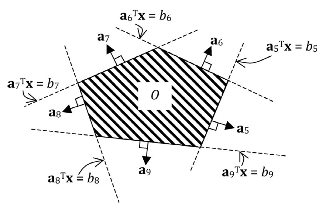
Polygonal convex obstacles: outside of which state must remain. $$ \mathcal{O} \Longleftrightarrow \bigwedge_{t \in T(\mathcal{O})} \bigvee_{i \in G(\mathcal{O})} \mathbf{a}{i}^{\prime} \mathbf{x}{t} \geq b_{i} $$
Note that nonconvex obstacles can be created by composing several convex obstacles.
Problem formulation:
Problem 1: Chance-constrained path-planning problem: $$ \begin{array}= &{\min\limits_{\mathbf{u}{0}, \ldots, \mathbf{u}{k-1}} g\left(\mathbf{u}{0}, \ldots, \mathbf{u}{k-1}, \overline{\mathbf{x}}{0}, \ldots, \overline{\mathbf{x}}{k}\right)} \ {\text{subject to: }} \ &{\overline{\mathbf{x}}{k}=\mathbf{x}{\mathrm{goal}}} \ &{\mathbf{x}{t+1}=A \mathbf{x}{t}+B \mathbf{u}{t}+\omega{t}} \ &{\mathbf{x}{0} \sim \mathcal{N}\left(\hat{\mathbf{x}}{0}, P_{0}\right) \omega_{t} \sim \mathcal{N}(0, Q)} \ &{P \left( \left(\bigwedge_{i=1}^{N_{\mathcal{I}}} \mathcal{I}{i}\right) \wedge \left(\bigwedge{j=1}^{N_{O}} \mathcal{O}{j}\right) \right) \geq 1-\Delta} \end{array} $$ where $g(\cdot)$ is a piecewise linear cost function, $N{\mathcal{I}}$ and $N_{\mathcal{O}}$ are number of stay-in regions and obstacles. $\overline{\mathbb{x}}$ means the expectation of $\mathbb{x}$.
Difficulty of solving:
evaluating the chance constraint requires the computation of the integral of a multivariable Gaussian distribution over a finite, nonconvex region. This cannot be carried out in the closed form, and approximate techniques such as sampling are time consuming and introduce approximation error.
even if this integral could be computed efficiently, its value is nonconvex in the decision variables due to the disjunctions in $\mathcal{O}_i$ . $\longrightarrow$ the resulting optimization problem is intractable. A typical approach to dealing with nonconvex feasible spaces is the branch-and-bound method, which decomposes a nonconvex problem into a tree of convex problems. However, the branch-and-bound method cannot be directly applied, since the nonconvex chance constraint cannot be decomposed trivially into subproblems.
where $c_{ij}(X)$ are convex function of $X$. $n_{\text{dis}}$ and $n_{\text{cl}}$ are the number of disjunctions and clauses within each disjunction.
Disjunctive linear program:
Same as above, but the $f_{\text{eq}}(X)$ and $c_{ij}(X)$ are linear function of $X$.
Difficulty of disjunctive convex program:
disjunction render the feasible region nonconvex. Nonconvex programs are intractable.
Method:
Decompose the problem into a finite number of convex subproblems. The number of convex subproblems is exponential in the number of disjunctions $n_{\text{dis}}$. Brach-and-bound can find the global optimal solution while solving only small subset.
Propogation
initial state: Gaussian $\mathcal{N}(\hat{\mathbb{x}}0, P_0)$ + dynamics : linear + noise: Gaussian $\longrightarrow$ future state is Gaussian $$ \begin{aligned} p(X_t|\mathbb{u}{0,\cdots,k-1}) &\sim \mathcal{N}(\mu_t,\Sigma_t)\ \mu_t & =\sum\limits_{i=0}^{t-1}A^{t-i-1}B\mathbb{u}_i + A^t \hat{\mathbb{x}}0 \quad {\text{linear equation}}\ \sum_t &= \sum\limits{t=0}^{t-1} A^iQ(A^T)^i + A^tP_0(A^T)^t \quad {\text{not about control inputs}} \end{aligned} $$
Linear Chance Constraints as Deterministic Linear Constraints
erf: $\operatorname{erf}(x) = \frac{2}{\sqrt{\pi}} \int\limits_0^x e^{-t^2} dt$ (gives the probability of a random variable with normal distribution of mean 0 and variance 1/2 falling in the range $[-x,x]$)
Gaussian form translation: $f(x|\mu,\sigma^2)=\frac{1}{\sigma} \varphi(\frac{x-\mu}{\sigma})$
Chance-constrained Collision Avoidance for MAVs in Dynamics Environments
Chance-constrained nonlinear model predictive control (CCNMPC)
assume uncertainties as Gaussian distribution, transform chance constraints into deterministic constraints
Model:
robot model: $$ \mathbf{x}{i}^{k+1}=\mathbf{f}{i}\left(\mathbf{x}{i}^{k}, \mathbf{u}{i}^{k}\right)+\omega_{i}^{k}, \quad \mathbf{x}{i}^{0} \sim \mathcal{N}\left(\hat{\mathbf{x}}{i}^{0}, \Gamma_{i}^{0}\right),\quad \omega_i^k\sim\mathcal{N}(0,Q_i^k) $$ where $\mathbf{x}{i}^{k}=\left[\mathbf{p}{i}^{k}, \mathbf{v}{i}^{k}, \phi{i}^{k}, \theta_{i}^{k}, \psi_{i}^{k}\right]^{T} \in \mathcal{X}{i} \subset \mathbb{R}^{n{x}}$, the mean and covariance of initial state$\mathbf{x}_i^0$ are obtained by state estimator (UKF).
Obstacle model:
$o\in \mathcal{I}_0={1,2,\cdots,n_0} \subset \mathbb{N}$ at position $\mathbf{p}_o \in \mathbb{R}^3$, can be represented by ellipsoid $S_0$ with semi-principal axes $(a_0,b_o,c_o)$ and rotation matrix $R_o$.
moving obstacles has constant velocity with Gaussian noise $\omega_o(t)\sim\mathcal{N}(0,Q_o(t))$ in acceleration, i.e. $\ddot{\mathbf{p}}_o=\omega_o(t)$. estimate and predict the future position and uncertainty by linear KF.
Collision Chance Constraints:
Collision condition:
collision of robot $i$ with robot $j$ $$ C_{i j}^{k} :=\left{\mathbf{x}{i}^{k} |\left|\mathbf{p}{i}^{k}-\mathbf{p}{j}^{k}\right| \leq r{i}+r_{j}\right} $$
collision of robot $i$ with obstacle $o$:
obstacle: enlarged ellipsoid and check if the robot is inside it. $$ C_{i o}^{k} :=\left{\mathbf{x}{i}^{k} |\left|\mathbf{p}{i}^{k}-\mathbf{p}{o}^{k}\right|{\Omega_{i o}} \leq 1\right},\quad \Omega_{i o}=R_{o}^{T} \operatorname{diag}\left(1 /\left(a_{o}+r_{i}\right)^{2}, 1 /\left(b_{o}+r_{i}\right)^{2}, 1 /\left(c_{o}+r_{i}\right)^{2}\right) {R_{o}} $$
optimization problem with $N$ time steps and planning horizon $\tau=N\Delta t$, $\Delta t$ is time step. $$ \begin{aligned} \min {\hat{x}{i}^{1}, \cdots, u_{i}^{0}, N-1} \quad & \sum_{k=0}^{N-1} J_{i}^{k}\left(\hat{\mathbf{x}}{i}^{k}, \mathbf{u}{i}^{k}\right)+J_{i}^{N}\left(\hat{\mathbf{x}}{i}^{N}\right) \ \text { s.t. }\quad & \mathbf{x}{i}^{0}=\hat{\mathbf{x}}{i}(0), \quad \hat{\mathbf{x}}{i}^{k}=\mathbf{f}{i}\left(\hat{\mathbf{x}}{i}^{k-1}, \mathbf{u}{i}^{k-1}\right) \ & \operatorname{Pr}\left(\mathbf{x}{i}^{k} \notin C_{i j}^{k}\right) \geq 1-\delta_{r}, \forall j \in \mathcal{I}, j \neq i \ & \operatorname{Pr}\left(\mathbf{x}{i}^{k} \notin C{i o}^{k}\right) \geq 1-\delta_{o}, \forall o \in \mathcal{I}{o} \ & \mathbf{u}{i}^{k-1} \in \mathcal{U}{i}, \quad \hat{\mathbf{x}}{i}^{k} \in \mathcal{X}_{i} \ & \forall k \in{1, \ldots, N} \end{aligned} $$
Compute uncertainty propagation
Methods:
Y. Z. Luo and Z. Yang, “A review of uncertainty propagation in orbital mechanics,” Progr. Aerosp. Sci., vol. 89, pp. 23–39, 2017.
Unscented transformation
A.Vo ̈lzandK.Graichen,“Stochastic model predictive control of nonlinear continuous-time systems using the unscented transformation,” inProc. Eur. Control Conf., 2015, pp. 3365–3370.
polynomial chaos expansions
A. Mesbah, S. Streif, R. Findeisen, and R. D. Braatz, “Stochastic nonlinear model predictive control with probabilistic constraints,” in Proc. Amer. Control Conf., 2014, pp. 2413–2419.
These methods are computational intensive and only outperform linearization methods when the propagation time is very long.
In this paper, propagate the uncertainty using EKF-type update. $$ \Gamma_{i}^{k+1}={F_{i}^{k}} {\Gamma_{i}^{k}} {F_{i}^{k}}^{T}+Q_{i}^{k} $$ ${\Gamma_{i}^{k}}$ is the state uncertainty covariance at time $k$, $F_{i}^{k}=\left.\frac{\partial \mathbf{f}{i}}{\partial \mathbf{x}{i}}\right|{\hat{\mathbf{x}}{i}^{k-1}, \mathbf{u}_{i}^{k}}$ is the state transition matrix of robot.
Chance Constraints:
Idea: linearize the collision conditions to get linear chance constraints. Then reformulate them into deterministic constraints
Linear Constraints: $$ \operatorname{Pr}(\mathbf{a}^T \mathbf{x}\leq b) \leq \delta $$ $\mathbf{x}$ Follows Gaussian distribution, the chance constraint can be transformed into deterministic constraint
Lemma 1:
Given a multivariate random variable $\mathbf{x}\sim\mathcal{N}(\hat{\mathbf{x}},\Sigma)$, then $$ \operatorname{Pr}\left(\mathbf{a}^{T} \mathbf{x} \leq b\right)=\frac{1}{2}+\frac{1}{2} \operatorname{erf}\left(\frac{b-\mathbf{a}^{T} \hat{\mathbf{x}}}{\sqrt{2 \mathbf{a}^{T} \Sigma \mathbf{a}}}\right) $$ where $\operatorname{erf}(\cdot)$ is standard error function as $\operatorname{erf}(x)=\frac{2}{\sqrt{\pi}}\int_0^x e^{-t^2} dt$.
Lemma 2:
Given a multivariate random variable $\mathbf{x}\sim\mathcal{N}(\hat{\mathbf{x}},\Sigma)$ and a probability threshold $\delta\in(0,0.5)$, then $$ \operatorname{Pr}\left(\mathbf{a}^{T} \mathbf{x} \leq b\right) \leq \delta \Longleftrightarrow \mathbf{a}^{T} \hat{\mathbf{x}}-b \geq c $$ where $c=\operatorname{erf}^{-1}(1-2 \delta) \sqrt{2 \mathbf{a}^{T} \Sigma \mathbf{a}}$.
erf: $\operatorname{erf}(x) = \frac{2}{\sqrt{\pi}} \int\limits_0^x e^{-t^2} dt$ (gives the probability of a random variable with normal distribution of mean 0 and variance 1/2 falling in the range $[-x,x]$)
Gaussian form translation: $f(x|\mu,\sigma^2)=\frac{1}{\sigma} \varphi(\frac{x-\mu}{\sigma})$
Inter-robot Collision Avoidance Constraint
Two robot position $\mathbf{p}{i} \sim \mathcal{N}\left(\hat{\mathbf{p}}{i}, \Sigma_{i}\right)$, $\mathbf{p}{j} \sim \mathcal{N}\left(\hat{\mathbf{p}}{j}, \Sigma_{j}\right)$, the collision probability is $$ \operatorname{Pr}\left(\mathbf{x}{i} \in C{i j}\right)=\int_{\mathbb{R}^{3}} I_{C}\left(\mathbf{p}{i}, \mathbf{p}{j}\right) p\left(\mathbf{p}{i}\right) p\left(\mathbf{p}{j}\right) d \mathbf{p}{i} d \mathbf{p}{j} $$ where $I_C$ is the indicator function, i.e., $$ I_{C}\left(\mathbf{p}{i}, \mathbf{p}{j}\right)=\left{\begin{array}{ll}{1,} & {\text { if }\left|\mathbf{p}{i}-\mathbf{p}{j}\right| \leq r_{i}+r_{j}} \ {0,} & {\text { otherwise }}\end{array}\right. $$
Assume $\mathbf{p}{i}$ and $\mathbf{p}{j}$ independent. $\mathbf{p}{i}-\mathbf{p}{j}\sim \mathcal{N}\left({\mathbf{p}{i}}-{\mathbf{p}{j}}, \Sigma_{i}-\Sigma_{j} \right)$, so $$ \operatorname{Pr}\left(\mathbf{x}{i} \in C{i j}\right)=\int_{\left|\mathbf{p}{i}-\mathbf{p}{j}\right| \leq r_{i}+r_{j}} p\left(\mathbf{p}{i}-\mathbf{p}{j}\right) d\left(\mathbf{p}{i}-\mathbf{p}{j}\right). $$
Here, Collision region is a sphere, and the distribution of $\mathbf{p}_{ij}$ is a ellipsoid. Hard to compute.
Transform the spherical collision region $C_{ij}$ into half space $\tilde{C}_{ij}$ $$ \tilde{C}{i j} :=\left{\mathbf{x} | \mathbf{a}{i j}^{T}\left(\mathbf{p}{i}-\mathbf{p}{j}\right) \leq b_{i j}\right} $$ where $\mathbf{a}{i j}=\left(\hat{\mathbf{p}}{i}-\hat{\mathbf{p}}{j}\right) /\left|\hat{\mathbf{p}}{i}-\hat{\mathbf{p}}{j}\right| \text { and } b{i j}=r_{i}+r_{j}$
Based on Lemma 1, an upper bound can be obtained: $$ \operatorname{Pr}\left(\mathbf{x}{i} \in C{i j}\right) \leq \frac{1}{2}+\frac{1}{2} \operatorname{erf}\left(\frac{b_{i j}-\mathbf{a}{i j}^{T}\left(\hat{\mathbf{p}}{i}-\hat{\mathbf{p}}{j}\right)}{\sqrt{2 \mathbf{a}{i j}^{T}\left(\Sigma_{i}+\Sigma_{j}\right) \mathbf{a}{i j}}}\right) $$ Based on Lemma 2, transform the chance constraint into deterministic constraint: $$ \mathbf{a}{i j}^{T}\left(\hat{\mathbf{p}}{i}-\hat{\mathbf{p}}{j}\right)-b_{i j} \geq \operatorname{erf}^{-1}\left(1-2 \delta_{r}\right) \sqrt{2 \mathbf{a}{i j}^{T}\left(\Sigma{i}+\Sigma_{j}\right) \mathbf{a}_{i j}} $$
Robot-Obstacle Collision Chance constraint
position of robots and obstacles are independent. $$ \operatorname{Pr}\left(\mathbf{x}{i} \in C{i o}\right)=\int_{\left|\mathbf{p}{i}-\mathbf{p}{o}\right|{\Omega{i o}} \leq 1} p\left(\mathbf{p}{i}-\mathbf{p}{o}\right) d\left(\mathbf{p}{i}-\mathbf{p}{o}\right) $$ Here, collision region is ellipsoid.
Linearize the collision
Affine coordinate transformation $\tilde{\mathbf{y}}=\Omega_{jo}^{\frac{1}{2}} \mathbf{y}$ to transform ellipsoid to unit sphere $\tilde{C}_{io}$. Accordingly, the robot and obstacel position need to be transformed into new distribution
$\tilde{\mathbf{p}}{i} \sim \mathcal{N}\left(\hat{\tilde{\mathbf{p}}}{i}, \tilde{\Sigma}{i}\right)$, $\tilde{\mathbf{p}}{o} \sim \mathcal{N}\left(\hat{\mathbf{p}}{o}, \tilde{\Sigma}{o}\right)$, where $$ \begin{aligned} \hat{\mathbf{p}}{i}=\Omega{i o}^{\frac{1}{2}} \hat{\mathbf{p}}{i}, & \tilde{\Sigma}{i}=\Omega_{i o}^{\frac{1}{2} T} \Sigma_{i} \Omega_{i o}^{\frac{1}{2}} \ \hat{\hat{\mathbf{p}}}{o}=\Omega{i o}^{\frac{1}{2}} \hat{\mathbf{p}}{o}, & \tilde{\Sigma}{o}=\Omega_{i o}^{\frac{1}{2} T} \Sigma_{o} \Omega_{i o}^{\frac{1}{2}} \end{aligned} $$ let $\operatorname{Pr}\left(\tilde{\mathbf{x}}{i} \in \tilde{C}{i o}\right)=\int_{\left|\mathbb{D}{i}-\tilde{\mathbf{p}}{o}\right| \leq 1} p\left(\tilde{\mathbf{p}}{i}-\tilde{\mathbf{p}}{o}\right) d\left(\tilde{\mathbf{p}}{i}-\tilde{\mathbf{p}}{o}\right) $, we have $$ \operatorname{Pr}\left(\mathbf{x}{i} \in C{i o}\right)=\operatorname{Pr}\left(\tilde{\mathbf{x}}{i} \in \tilde{C}{i o}\right) $$ Use same linearization method for phere with $\mathbf{a}{i o}=\left(\hat{\mathbf{p}}{i}-\hat{\mathbf{p}}{o}\right) /\left|\hat{\mathbf{p}}{i}-\hat{\mathbf{p}}{o}\right| \text { and } b{i o}=1$.
Model each robot as enclosing rigid sphere $S_i$ with radius $r_i$, $i$ means the index of robots $i\in{1, 2, \cdots,n}$. $$ x_i^{k+1}=f_i(x_i^{k})+B u_i^{k} + \omega_i^k, \quad x_i^k \sim \mathcal{N}(\hat{x}_i^0,\Gamma_i^0), \quad \omega_i^k\sim\mathcal{N}(0,Q_i^k) $$ Mean $\hat{x}_i^0$ and covariance $\Gamma_i^0$ of initial state can be estimated by UKF. State $x_i^k = [(p_i^k)^\top, (v_i^k)^\top, (\zeta_i^k)^\top, (\omega_i^k)^\top ]^\top.$
Moving Obstacle model:
obstacle $o \in {1, 2, \cdots, m}$ at position $p_o$, modelling it as non-rotating ellipsoid $S_o$ with semi-principal axes $(a_0,b_0,c_0)$ and rotation matrix $R_o$.
Constant velocity with noise $\omega_o(t)\sim\mathcal{N}(0, Q_o(t))$, i.e., $\dot{p}_o(t)=\omega_o(t)$.
predict its future position using KF.
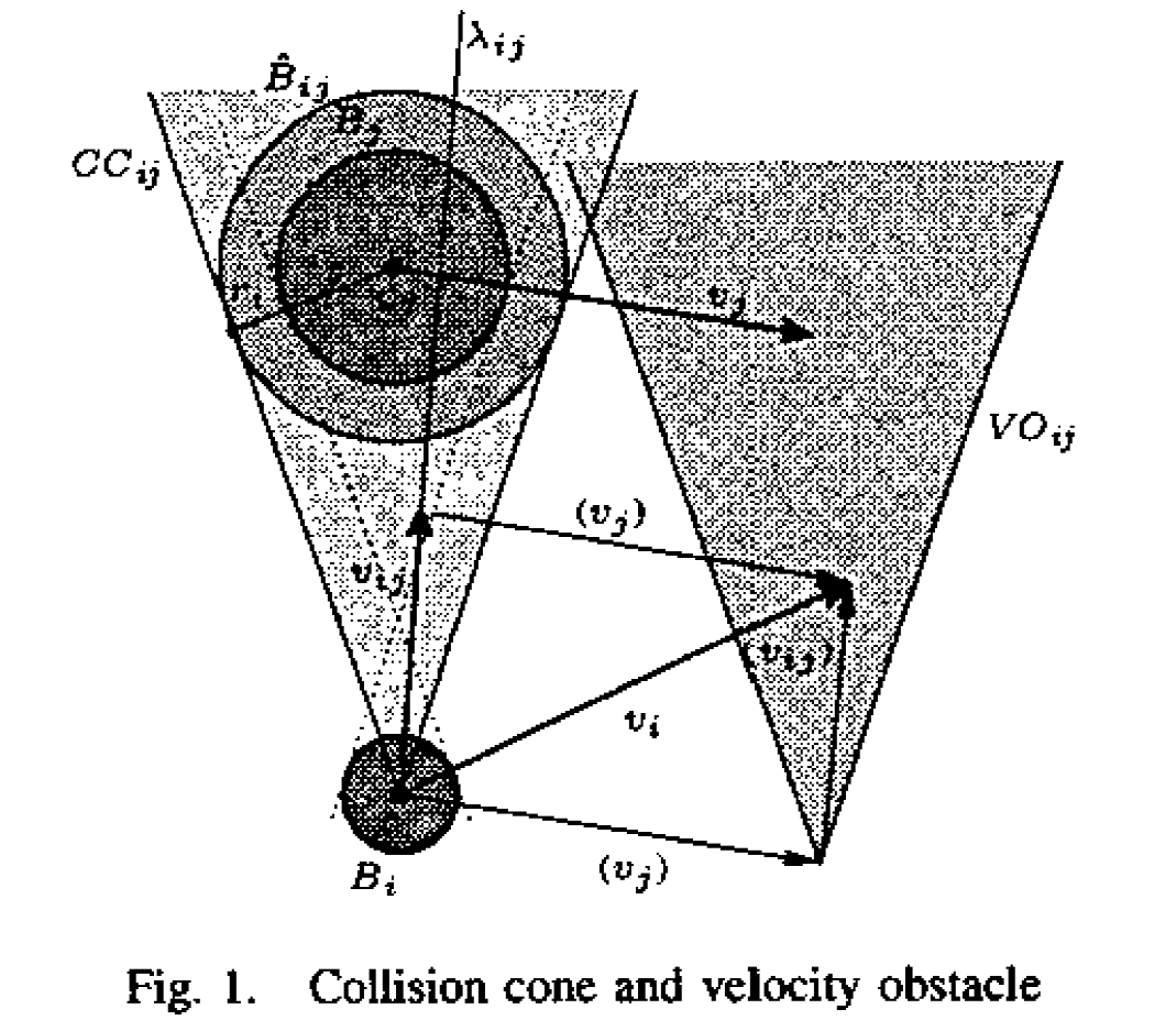
Velocity Obstacles:
robot $B_i$ is circle, center $c_i$, radius $r_i$, velocity $v_i=\dot{c}_i$
robot $B_j$ is circle, center $c_j$, radius $r_j$, velocity $v_j = \dot{c}_j$
pdf of velocity of $B_{j}$ : $V_j: \mathbb{R}^2 \rightarrow \mathbb{R}_0^+$
==Probabilistic velocity obstacles==: $PVO_{ij}: \mathbb{R}^2 \rightarrow [0,1]$ $$ PVO_{ij} (v_i) = \int\limits_{R^2} V_j(v_j) \ PCC_{ij}(v_i-v_j) \ d^2v_j $$ which is equivalent to $$ PVO_{ij} (v_i) = V_j * \ PCC_{ij} \quad \text{convolution of two function} $$ Composite Probabilistic Velocity Obstacle $$ PVO_i = 1 - \prod\limits_{j\neq i} \left(1-PVO_{ij}\right) $$ ==Navigation:==
$U_i : \mathbb{R}^2 \rightarrow [0,1]$ : utility of velocities $v_i$ for the motion goal of $B_i$. Full utility of $v_i$ is only attained if (1) $v_i$ is dynamically reachable (2) $v_i$ is collision free.
relative utility function: $$ RU_i = U_i \cdot D_i \cdot (1-PVO_i) $$ $D_i : \mathbb{R}^2 \rightarrow [0,1]$ means reachability of a new velocity.
Repeatedly choose a velocity $v_i$ which maximizes the relative utility $RU_i$.
$$ \mathbf{x}{i}^{k+1}=\mathbf{f}{i}\left(\mathbf{x}{i}^{k}, \mathbf{u}{i}^{k}\right)+\omega_{i}^{k}, \quad \mathbf{x}{i}^{0} \sim \mathcal{N}\left(\hat{\mathbf{x}}{i}^{0}, \Gamma_{i}^{0}\right),\quad \omega_i^k\sim\mathcal{N}(0,Q_i^k) $$ where $\mathbf{x}{i}^{k}=\left[\mathbf{p}{i}^{k}, \mathbf{v}{i}^{k}, \phi{i}^{k}, \theta_{i}^{k}, \psi_{i}^{k}\right]^{T} \in \mathcal{X}{i} \subset \mathbb{R}^{n{x}}$, the mean and covariance of initial state $\mathbf{x}_i^0$ are obtained by state estimator (UKF).
Obstacle model:
$o\in \mathcal{I}_0={1,2,\cdots,n_0} \subset \mathbb{N}$ at position $\mathbf{p}_o \in \mathbb{R}^3$, can be represented by ellipsoid $S_0$ with semi-principal axes $(a_0,b_o,c_o)$ and rotation matrix $R_o$.
moving obstacles has constant velocity with Guassian noise $\omega_o(t)\sim\mathcal{N}(0,Q_o(t))$ in aaceleration, i.e. $\ddot{\mathbf{p}}_o=\omega_o(t)$. estimate and predict the future position and uncertainty by linear KF.
Collision Chance Constraints:
Collision condition:
collision of robot $i$ with robot $j$ $$ C_{i j}^{k} :=\left{\mathbf{x}{i}^{k} |\left|\mathbf{p}{i}^{k}-\mathbf{p}{j}^{k}\right| \leq r{i}+r_{j}\right} $$
collision of robot $i$ with obstacle $o$:
obstacle: enlarged ellipsoid and check if the robot is inside it. $$ C_{i o}^{k} :=\left{\mathbf{x}{i}^{k} |\left|\mathbf{p}{i}^{k}-\mathbf{p}{o}^{k}\right|{\Omega_{i o}} \leq 1\right},\quad \Omega_{i o}=R_{o}^{T} \operatorname{diag}\left(1 /\left(a_{o}+r_{i}\right)^{2}, 1 /\left(b_{o}+r_{i}\right)^{2}, 1 /\left(c_{o}+r_{i}\right)^{2}\right) {R_{o}} $$
Approximate continuous curve by a piecewise linear cure. In order to have good approximation, we need sufficient pieces (basic components of the piecewise linear curve).
sigmoid: $y(x;c,b,w)=c\frac{1}{1+e^{-(b+wx)}}$
How to reduce the model bias:
more flexible model
more feature
In ML, the pieces (activation function) can be sigmoid function, hard sigmoid, ReLU, etc.
number of hidden layer
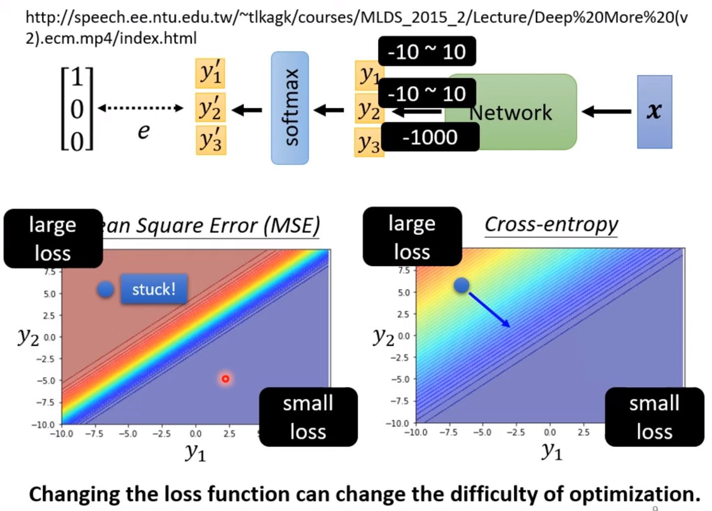
2. Define Loss $L(\theta)$
Loss: function of parameters to evaluate how good of the set of parameters $L=\frac{1}{N} \sum_n e_n$.
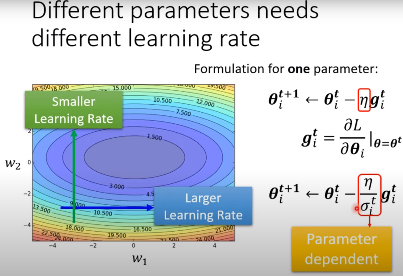
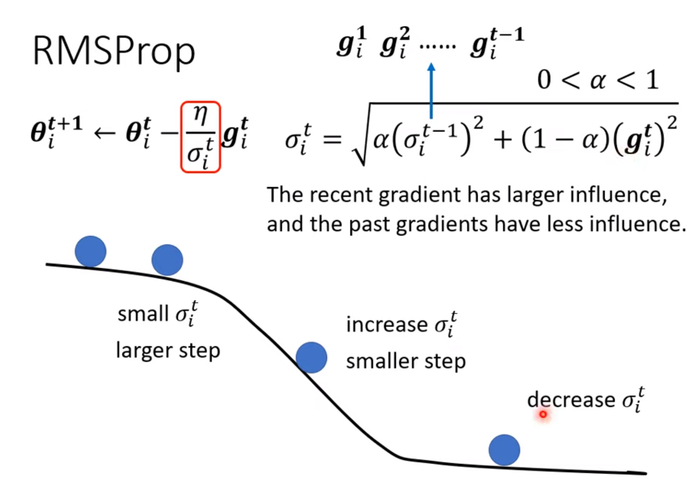
learning rate decay: As the time goes, we are closer to the destination, so we reduce the learning rate
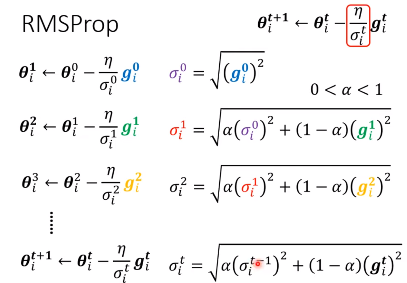
warm up: increase first and then decrease (at the beginning, the estimate of $\sigma_i^t$ has large variance) [RAdam]
Problem:
overfitting
Methods to improve:
reason of large loss on training data:
Model bias: model is too simple. –> redesign more flexible model (more feature; more neutrons layers)
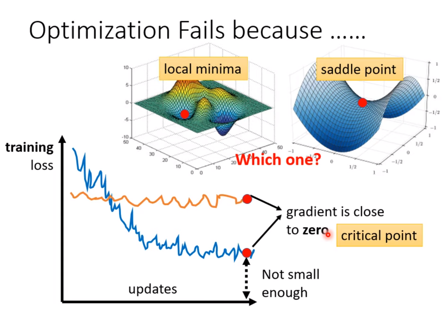
Optimization: local minima
How to know which reason leads to the large loss on training data:
If deeper network has larger loss on training data, there might be optimization issue.
Overfitting:
Smaller loss on training data, and larger loss on testing data.
Solution:
more training data;
Data augmentation (reasonable);
constrained model
less parameters, sharing parameters [e.g. CNN which is constrained one compared with fully-connected NN]
Less features
early stopping
regularization
Dropout
But if give more constraints on model, –> Bias-complexity trade-off [cross validation, N-fold cross validation]
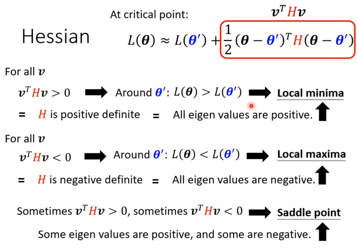
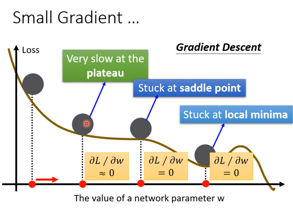
critical point: gradient = 0
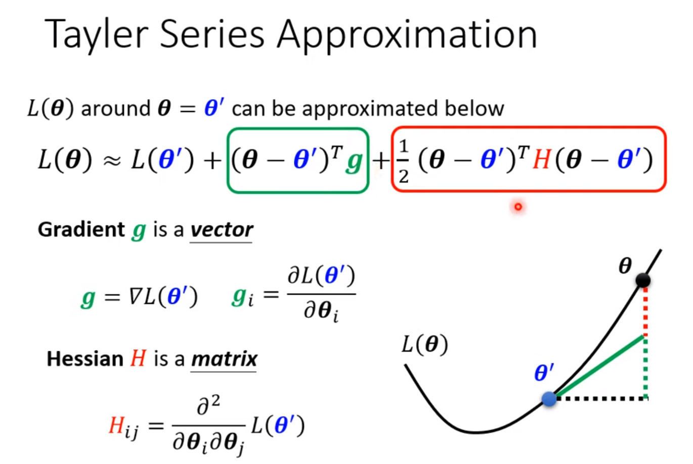
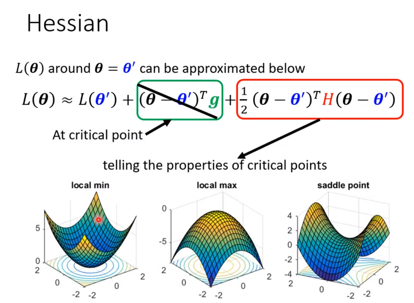
把data的loss写出来,求loss对每个参数的偏导,令其=0, 检测其Hessian
How to avoid critical point ?
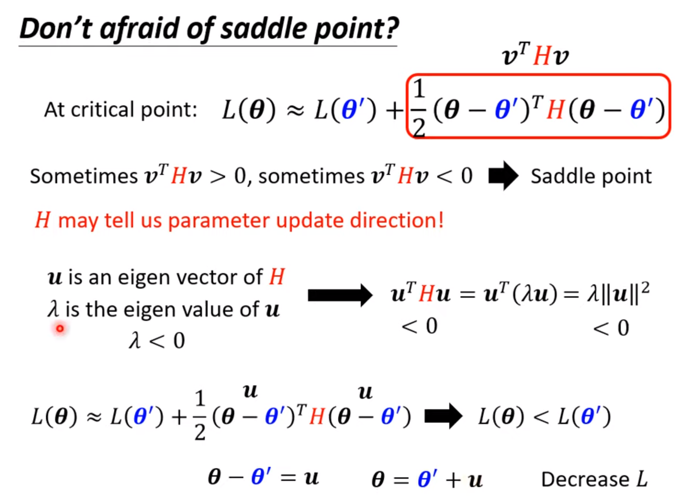
Avoid saddle point
Based on eigenvector and eigenvalue of Hessian, we can update the parameter along the direction of the eigenvector –> reduce loss.
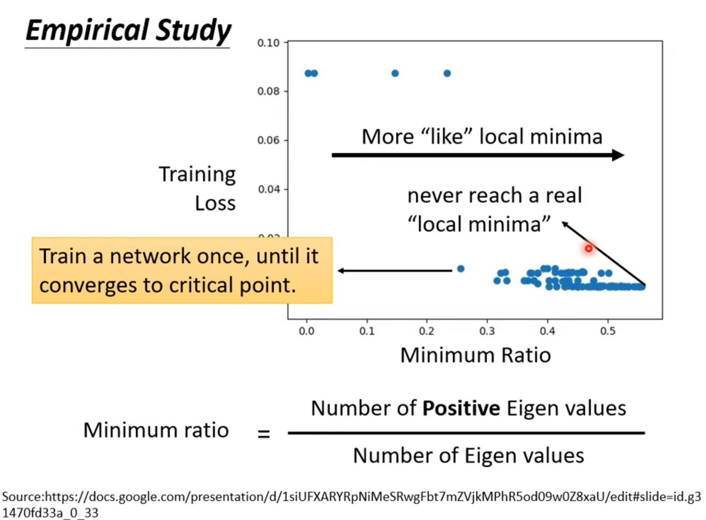
If enough more parameter, the error surface will be more complex. But the local minima will be degrade to saddle point. [local minima in low dimension –> saddle point in higher dimension].