Chance-constrained ADD Velocity Obstacles
Chance-constrained + Velocity Obstacles
Model:
Original robot model:
$$
\dot{x}=f(x)+B u
$$
In detail,
$$
\begin{equation}
\label{eq:model}
\begin{bmatrix} {\dot{p}} \ {\dot{v}} \ {\dot{\zeta}} \ {\dot{\omega}}\end{bmatrix} =
\begin{bmatrix} {R(\phi, \theta, \psi)}^\top {v} \ {-{\omega}\times v + g {R(\phi, \theta, \psi)} e} \ W(\phi, \theta, \psi) {\omega} \ J^{-1}(-{\omega} \times J {\omega}) \end{bmatrix} + B {(u_{eq} + \delta u)}. \
\end{equation}
$$
with ${e}=[0,0,1]^\top$,
$$
{R}(\phi, \theta, \psi)=
\begin{bmatrix}
{c\theta c\psi} & {c\theta s\psi} & {-s\theta} \
{s\theta c\psi s\phi-s\psi c\phi} & {s\theta s\psi s\phi+c\psi c\phi} & {c\theta s\phi} \
{s\theta c\psi c\phi+s\psi s\phi} & {s\theta s\psi c\phi-c\psi s\phi} & {c\theta c\phi}
\end{bmatrix}.
$$
and
$$
\begin{equation*}
W(\phi, \theta, \psi)=\begin{bmatrix}{1} & {s\phi t\theta} & {c\phi t\theta} \ {0} & {c\phi} & {-s\phi} \ {0} & {s\phi sc\theta} & {c\phi sc\theta}\end{bmatrix}.
\end{equation*}
$$Stochastic Robot model:
Model each robot as enclosing rigid sphere $S_i$ with radius $r_i$, $i$ means the index of robots $i\in{1, 2, \cdots,n}$.
$$
x_i^{k+1}=f_i(x_i^{k})+B u_i^{k} + \omega_i^k, \quad x_i^k \sim \mathcal{N}(\hat{x}_i^0,\Gamma_i^0), \quad \omega_i^k\sim\mathcal{N}(0,Q_i^k)
$$
Mean $\hat{x}_i^0$ and covariance $\Gamma_i^0$ of initial state can be estimated by UKF. State $x_i^k = [(p_i^k)^\top, (v_i^k)^\top, (\zeta_i^k)^\top, (\omega_i^k)^\top ]^\top.$Moving Obstacle model:
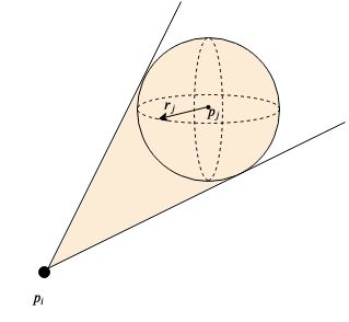
obstacle $o \in {1, 2, \cdots, m}$ at position $p_o$, modelling it as non-rotating ellipsoid $S_o$ with semi-principal axes $(a_0,b_0,c_0)$ and rotation matrix $R_o$.
Constant velocity with noise $\omega_o(t)\sim\mathcal{N}(0, Q_o(t))$, i.e., $\dot{p}_o(t)=\omega_o(t)$.
predict its future position using KF.
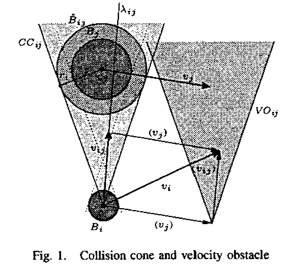
Velocity Obstacles:
robot $B_i$ is circle, center $c_i$, radius $r_i$, velocity $v_i=\dot{c}_i$
robot $B_j$ is circle, center $c_j$, radius $r_j$, velocity $v_j = \dot{c}_j$
relative velocity $v_{ij} = v_i - v_j$
Collision region:
$$
B_{ij} = { c_j + r: r\in R^2, |r| \leq r_i+r_j }
$$$$
\lambda_{ij}(v_{ij}) = {c_i+\mu v_{ij}: \mu\geq0}
$$Collision occurs iff $B_{ij}\cap \lambda_{ij}(v_{ij}) \ne \empty$
Collision cone $CC_{ij}$
$$
CC_{ij} = { v_{ij}:B_{ij}\cap\lambda_{ij}(v_{ij})\neq \empty }
$$Velocity Obstacle $VO_{ij}$
$$
VO_{ij} = { v_i: (v_i-v_j)\in CC_{ij} }
$$
i.e., $VO_{ij} = v_j + CC_{ij}$Now, for $B_i$, any velocity $v_i\in VO_{ij}$ will lead to collision.
Composite velocity obstacle for $B={B_1, \cdots, B_n}$
$$
VO_i=\cup_{j\ne i} VO_{ij}
$$
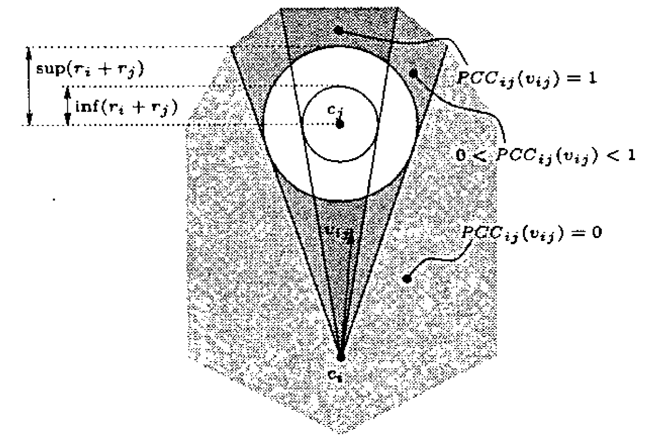
Probabilistic Velocity Obstacles
- uncertainty of shape and velocity
Shape uncertainty
probabilistic collision cone : $PCC_{ij}: \mathbb{R}^2 \rightarrow [0,1]$
Velocity Uncerinty
pdf of velocity of $B_{j}$ : $V_j: \mathbb{R}^2 \rightarrow \mathbb{R}_0^+$
==Probabilistic velocity obstacles==: $PVO_{ij}: \mathbb{R}^2 \rightarrow [0,1]$
$$
PVO_{ij} (v_i) = \int\limits_{R^2} V_j(v_j) \ PCC_{ij}(v_i-v_j) \ d^2v_j
$$
which is equivalent to
$$
PVO_{ij} (v_i) = V_j * \ PCC_{ij} \quad \text{convolution of two function}
$$
Composite Probabilistic Velocity Obstacle
$$
PVO_i = 1 - \prod\limits_{j\neq i} \left(1-PVO_{ij}\right)
$$
==Navigation:==$U_i : \mathbb{R}^2 \rightarrow [0,1]$ : utility of velocities $v_i$ for the motion goal of $B_i$. Full utility of $v_i$ is only attained if (1) $v_i$ is dynamically reachable (2) $v_i$ is collision free.
relative utility function:
$$
RU_i = U_i \cdot D_i \cdot (1-PVO_i)
$$
$D_i : \mathbb{R}^2 \rightarrow [0,1]$ means reachability of a new velocity.Repeatedly choose a velocity $v_i$ which maximizes the relative utility $RU_i$.
Collision Chance Constraints:
robot $i$: position $p_i$, velocity $v_i$
robot $j$: position $p_j$, velocity $v_j$
- Collision Condition:
$$
C_{ij}^k := { v_i^k \lvert | v_i^k-v_j^k | }
$$
- Collision Condition:
$$
\mathbf{x}{i}^{k+1}=\mathbf{f}{i}\left(\mathbf{x}{i}^{k}, \mathbf{u}{i}^{k}\right)+\omega_{i}^{k}, \quad \mathbf{x}{i}^{0} \sim \mathcal{N}\left(\hat{\mathbf{x}}{i}^{0}, \Gamma_{i}^{0}\right),\quad \omega_i^k\sim\mathcal{N}(0,Q_i^k)
$$
where $\mathbf{x}{i}^{k}=\left[\mathbf{p}{i}^{k}, \mathbf{v}{i}^{k}, \phi{i}^{k}, \theta_{i}^{k}, \psi_{i}^{k}\right]^{T} \in \mathcal{X}{i} \subset \mathbb{R}^{n{x}}$, the mean and covariance of initial state $\mathbf{x}_i^0$ are obtained by state estimator (UKF).
Obstacle model:
$o\in \mathcal{I}_0={1,2,\cdots,n_0} \subset \mathbb{N}$ at position $\mathbf{p}_o \in \mathbb{R}^3$, can be represented by ellipsoid $S_0$ with semi-principal axes $(a_0,b_o,c_o)$ and rotation matrix $R_o$.
moving obstacles has constant velocity with Guassian noise $\omega_o(t)\sim\mathcal{N}(0,Q_o(t))$ in aaceleration, i.e. $\ddot{\mathbf{p}}_o=\omega_o(t)$. estimate and predict the future position and uncertainty by linear KF.
Collision Chance Constraints:
Collision condition:
collision of robot $i$ with robot $j$
$$
C_{i j}^{k} :=\left{\mathbf{x}{i}^{k} |\left|\mathbf{p}{i}^{k}-\mathbf{p}{j}^{k}\right| \leq r{i}+r_{j}\right}
$$collision of robot $i$ with obstacle $o$:
obstacle: enlarged ellipsoid and check if the robot is inside it.
$$
C_{i o}^{k} :=\left{\mathbf{x}{i}^{k} |\left|\mathbf{p}{i}^{k}-\mathbf{p}{o}^{k}\right|{\Omega_{i o}} \leq 1\right},\quad
\Omega_{i o}=R_{o}^{T} \operatorname{diag}\left(1 /\left(a_{o}+r_{i}\right)^{2}, 1 /\left(b_{o}+r_{i}\right)^{2}, 1 /\left(c_{o}+r_{i}\right)^{2}\right) {R_{o}}
$$
Chance constraints:
$$
\begin{array}{ll}{\operatorname{Pr}\left(\mathbf{x}{i}^{k} \notin C{i j}^{k}\right) \geq 1-\delta_{r},} & {\forall j \in \mathcal{I}, j \neq i} \ {\operatorname{Pr}\left(\mathbf{x}{i}^{k} \notin C{i o}^{k}\right) \geq 1-\delta_{o},} & {\forall o \in \mathcal{I}_{o}}\end{array}
$$
Problem Formulation:
optimiation problem with $N$ time steps and planning horizon $\tau=N\Delta t$, $\Delta t$ is time step.
$$
\begin{aligned} \min {\hat{x}{i}^{1}, \cdots, u_{i}^{0}, N-1} \quad & \sum_{k=0}^{N-1} J_{i}^{k}\left(\hat{\mathbf{x}}{i}^{k}, \mathbf{u}{i}^{k}\right)+J_{i}^{N}\left(\hat{\mathbf{x}}{i}^{N}\right) \ \text { s.t. }\quad & \mathbf{x}{i}^{0}=\hat{\mathbf{x}}{i}(0), \quad \hat{\mathbf{x}}{i}^{k}=\mathbf{f}{i}\left(\hat{\mathbf{x}}{i}^{k-1}, \mathbf{u}{i}^{k-1}\right) \ & \operatorname{Pr}\left(\mathbf{x}{i}^{k} \notin C_{i j}^{k}\right) \geq 1-\delta_{r}, \forall j \in \mathcal{I}, j \neq i \ & \operatorname{Pr}\left(\mathbf{x}{i}^{k} \notin C{i o}^{k}\right) \geq 1-\delta_{o}, \forall o \in \mathcal{I}{o} \ & \mathbf{u}{i}^{k-1} \in \mathcal{U}{i}, \quad \hat{\mathbf{x}}{i}^{k} \in \mathcal{X}_{i} \ & \forall k \in{1, \ldots, N} \end{aligned}
$$