Variational Inference
Variational Inference
The solution is obtained by exploring all possible input functions to find the one that maximizes, or minimizes, the functional.
restriction : factorization assumption
log marginal probability
$$
\ln p(\mathbf X) = \mathcal L(q)+ KL(q||p)
$$- This differs from our discussion of EM only in that the parameter vector $\theta$ no longer appears, because the parameters are now stochastic variables and are absorbed into $\mathbf Z$.
- maximize the lower bound $\mathcal L$ = minimize the KL divergence.
In particular, there is no ‘over-fitting’ associated with highly flexible distributions. Using more flexible approximations simply allows us to approach the true posterior distribution more closely.
- One way to restrict the family of approximating distributions is to use a parametric distribution $q(Z|ω)$ governed by a set of parameters $ω$. The lower bound $\mathcal L(q)$ then becomes a function of $ω$, and we can exploit standard nonlinear optimization techniques to determine the optimal values for the parameters.
Method:
Factorized distribution approximate to true posterior distribution –>> Mean field theory
$$
KL(p||q) \quad \iff \quad KL(q||p)
$$if we consider approximating a multimodal distribution by a unimodal one,
Both types of multimodality were encountered in Gaussian mixtures, where they manifested themselves as
multiple maxima in the likelihood function, and a variational treatment based on the minimization of $KL(q||p)$ will tend to find one of these modes.if we were to minimize $KL(p||q)$, the resulting approximations would average across all of the modes and, in the context of the mixture model, would lead to poor predictive distributions (because the average of two good parameter values is typically itself not a good parameter value). It is possible to make use of $KL(p||q)$ to define a useful inference procedure, but this requires a rather different approach about expectation propagation.
The two forms of KL divergence are members of the alpha family of divergence.
Variational Mixture of Gaussian
Likelihood function $p(\mathbf Z| \mathbf \pi) = \prod\limits_{n=1}^N \prod\limits_{k=1}^K \pi_k^{z_{nk}}$
Conditional distribution of observed data $p(\mathbf X|\mathbf Z,\mu, \Lambda) = \prod\limits_{n=1}^N \prod\limits_{k=1}^K \mathcal N(\mathbf x_n|\mu_k,\Lambda_k^{-1})^{z_{nk}}$
Prior distribution: $p(\pi) = \mathrm{Dir}(\pi|\alpha_0)$, $p(\mu,\Lambda) = p(\mu|\Lambda)p(\Lambda)=\prod\limits_{k=1}^N \mathcal N(\mu_k | m_0, (\beta_0\Lambda_k)^{-1}) \mathcal W(\Lambda_k|\mathbf W_0, \nu_0)$
Variables such as $\mathbb z_n$ that appear inside the plate are regarded as latent variables because the number of such variables grows with the size of the data set. By contrast, variables such as μ that are outside the plate are fixed in number independently of the size of the data set, and so are regarded as parameters
Variational distrbution
Joint distribution
$$
p(\mathbf{X}, \mathbf{Z}, \boldsymbol{\pi}, \boldsymbol{\mu}, \boldsymbol{\Lambda})=p(\mathbf{X} | \mathbf{Z}, \boldsymbol{\mu}, \boldsymbol{\Lambda}) p(\mathbf{Z} | \boldsymbol{\pi}) p(\boldsymbol{\pi}) p(\boldsymbol{\mu} | \boldsymbol{\Lambda}) p(\boldsymbol{\Lambda})
$$
Variational distribution (Assumption)
$$
q(\mathbf{Z}, \boldsymbol{\pi}, \boldsymbol{\mu}, \boldsymbol{\Lambda}) = q(\mathbf{Z})q(\boldsymbol{\pi}, \boldsymbol{\mu}, \boldsymbol{\Lambda})
$$
==Variational EM==
This effect can be understood qualitatively in terms of the automatic trade-off in a Bayesian model between fitting the data and the complexity of the model, in which the complexity penalty arises from components whose parameters are pushed away from their prior values.
Thus the optimization of the variational posterior distribution involves cycling between two stages analogous to the E and M steps of the maximum likelihood EM algorithm.
Variational E-step
use the current distributions over the model parameters to evaluate the moments in (10.64), (10.65), and (10.66)
and hence evaluate $\mathbb E[z_{nk}] = r_{nk}$.Variational M-step
keep these responsibilities fixed and use them to re-compute the variational distribution over the parameters using (10.57) and (10.59). In each case, we see that the variational posterior distribution has the same functional form as the corresponding factor in the joint distribution (10.41). This is a general result and is a consequence of the choice of conjugate distributions.
==variational EM v.s. EM for maximum likelihood.==
- In fact if we consider the limit $N\rightarrow \infty$ then the Bayesian treatment converges to the maximum likelihood EM algorithm.
- For anything other than very small data sets, the dominant computational cost of the variational algorithm for Gaussian mixturesa rises from the evaluation of the responsibilities, together with the evaluation and inversion of the weighted data covariance matrices. These computations mirror precisely those that arise in the maximum likelihood EM algorithm, and so there is little computational overhead in using this Bayesian approach as compared to the traditional maximum likelihood one.
- The singularities that arise in maximum likelihood when a Gaussian component ‘collapses’ onto a specific data point are absent in the Bayesian treatment. Indeed, these singularities are removed if we simply introduce a prior and then use a MAP estimate instead of maximum likelihood.
- Furthermore, there is no over-fitting if we choose a large number $K$ of components in the mixture.
- Finally, the variational treatment opens up the possibility of determining the optimal number of components in the mixture without resorting to techniques such as cross validation.
Variational lower bound
Function:
- to monitor the bound during the re-estimation in order to test for convergence
- provide a valuable check on both the mathematical expressions for the solutions and their software implementation, because at each step of the iterative re-estimation procedure the value of this bound should not decrease.
- provide a deeper test of the correctness of both the mathematical derivation of the update equations and of their software implementation by using finite differences to check that each update does indeed give a (constrained) maximum of the bound
lower bound provides an alternative approach for deriving the variational re-estimation equations in variational EM. To do
this we use the fact that, since the model has conjugate priors, the functional form of the factors in the variational posterior distribution is known, namely discrete for $\mathbf Z$, Dirichlet for $π$, and Gaussian-Wishart for $(μ_k,Λ_k)$. By taking general parametric forms for these distributions we can derive the form of the lower bound as a function of the parameters of the distributions. Maximizing the bound with respect to these parameters then gives the required re-estimation equations.
Predictive density
predictive density for a new value $\hat x$ of the observed variable. corresponding to latent variable $\hat{\mathbf z}$.
$$
p(\widehat{\mathbf{x}} | \mathbf{X})=\sum_{\widehat{\mathbf{z}}} \iiint p(\widehat{\mathbf{x}} | \widehat{\mathbf{z}}, \mu, \Lambda) p(\widehat{\mathbf{z}} | \boldsymbol{\pi}) p(\boldsymbol{\pi}, \boldsymbol{\mu}, \boldsymbol{\Lambda} | \mathbf{X}) \mathrm{d} \boldsymbol{\pi} \mathrm{d} \boldsymbol{\mu} \mathrm{d} \boldsymbol{\Lambda} \
= \sum_{k=1}^K \iiint \pi_k \mathcal N(\hat{\mathbf x} |\mu_k,\Lambda_k) q(\pi) q(\mu_k, \Lambda_k) d\pi d\mu_k d \Lambda_k
$$
remaining integrations can now be evaluated analytically giving a mixture of Student’s t-distributions:
$$
\begin{aligned}
p(\widehat{\mathbf{x}} | \mathbf{X})&= \frac{1}{\widehat{\alpha}} \sum_{k=1}^{K} \alpha_{k} \operatorname{St}\left(\widehat{\mathbf{x}} | \mathbf{m}{k}, \mathbf{L}{k}, \nu_{k}+1-D\right) \
\qquad \mathbf{L}{k}&=\frac{\left(\nu{k}+1-D\right) \beta_{k}}{\left(1+\beta_{k}\right)} \mathbf{W}_{k}
\end{aligned}
$$
where $\mathbf m_k$ is the mean of $k$th component.
Determining the number of components.
variational lower bound can be used to determine a posterior distribution over the number $K$ of components in the mixture model.
If we have a mixture model comprising $K$ components, then each parameter setting will be a member of a family of $K!$ equivalent settings.
- in EM, this is irrelevant because the parameter optimization algorithm will, depending on the initialization
of the parameters, find one specific solution, and the other equivalent solutions play no role. - in Variational EM, we marginalize over all possible parameter values.
- if the true posterior distribution is multimodal, variational inference based on the minimization of $KL(q||p)$ will tend to approximate the distribution in the neighborhood of one of the modes and ignore the others.
- If we want to compare different value of $K$, we need to consider the multimodality.
Solution:
- to add a term $\ln K!$ onto the lower bound when used for model comparison and averaging.
- treat the mixing coefficients $π$ as parameters and make point estimates of their values by maximizing the lower bound with respect to $π$ instead of maintaining a probability distribution over them as in the fully Bayesian approach.
- This leads to the re-estimation equation and this maximization is interleaved with the variational updates for the $q$ distribution over the remaining parameters.
- Components that provide insufficient contribution to explaining the data will have their mixing coefficients driven to zero during the optimization, and so they are effectively removed from the model through automatic relevance determination. This allows us to make a single training run in which we start with a relatively large initial value of K, and allow surplus components to be pruned out of the model.
==Comparison:==
- maximum likelihood would lead to values of the likelihood function that increase monotonically with K (assuming the singular solutions have been avoided, and discounting the effects of local maxima) and so cannot be used to determine an appropriate model complexity.
- By contrast, Bayesian inference automatically makes the trade-off between model complexity and fitting the data.
maximum likelihood would lead to values of the likelihood function that increase monotonically with K (assuming the singular solutions have been avoided, and discounting the effects of local maxima) and so cannot be used to determine an appropriate model complexity.
By contrast, Bayesian inference automatically makes the trade-off between model complexity and fitting the data.
Simplified description
Reference: 变分推断(Variational Inference)
Description
based on input data to compute a distribution $P(x)$.
Idea: Use Gaussian distribution can function as approximate distribution to simulate the real distribution
<用已知的分布模拟未知的分布>
Parameters:
- input: $x$
- hidden variable: $z$
- is parameter in real distribution. For GMM, $z$ is the mean and covariance of all gaussian distribution.
- Posterior distribution $P(z|x)$:
- using the data to guess the model. <用输入去推断隐含变量>
- likelihood distribution $P(x|z)$:
- distribution based on the model parameter.
- distribution of input $P(x)$
- Prior distribution $q(z,v)$:
- the distribution to simulate the real distribution. $z$ is hidden variables, $v$ is the parameter of distribution about $z$, i.e., hyperparameter.
- normally, the distribution about $z$ is conjugate distribution.
Task:
adjust $v$ to make the approximate distribution close to the posterior distribution $p(z|x)$
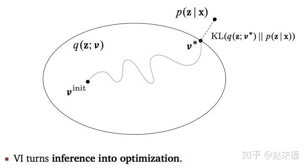
Hope the posterior distribution and the prior distribution closed to 0. But the posterior distribution is unknown. Therefore, introduce the KL divergence and ELBO.
$$
\log p(x) = KL(q(z;v) || p(z|x)) + ELBO(v)
$$
because $\log p(x)$ is constant, the minimum KL divergence is the maximum ELBO.