Chance-Constrained Optimal Path Planning with Obstacles
Chance-Constrained Optimal Path Planning with Obstacles
Prior works: Set-Bound Uncertainty
Key idea: use bounds on the probability of collision to approximate the nonconvex chance-constrained optimization problem as a disjunctive convex problem. Then, solve by Branch-and-Bound techniques.
Target: linearm discrete-time system.
UAV. Uncertainty:
location is not exactly known, but is estimated using a system model, interior sensors, and/or global position system. distribution may be generated with estimation technique, like KF.
$\rightarrow$ initial position is Gaussian distribution.
system model are approximations of true system model and these dynamixss are not fully known.
$\rightarrow$ model uncertainty to be Gaussian white noise
disturbances makes the turue trajecotyr. deviate from the palnned trajectory.
$\rightarrow$ modeled as Gaussian noise on dynamics.
Prior Method: Set-bounded uncertainty models. to make sure the disturbance do not exceed the bounds.
Chance Constraints:
- Advantages over set-bounded approach:
- disturbances are represented using a stochastic model, rather than set-bounded one.
- When use KF as localization, state estimate is a probabilsitic function with mean and covariancel
Existing CCP of linear system s.t. Gaussian uncertainty in convex region.
This paper extend to nonconvex region.
- Key: bound the probability of collision, give conservative approximation, formulate as disjunctive convex program, solve by Branch-and-Bound techniques.
Convex region:
Nonconvex region:
- Early, convert problem into set-bound by ensuring 3-$\sigma$ confidence region. Then, can solve. But fail to ding a feasible solution.
- Particle-based approach. Approximate the chance constraint, but not guarantee satisfaction of constraint. Can use arbitrary uncertainty distribution, rather than only Gaussian. But Computational intensive.
- Anylytic bound to ensure the satifaction of constraints. little conservatism.
System model:
$$
\mathbf{x}{t+1}=A \mathbf{x}{t}+B \mathbf{u}{t}+\omega{t}
$$
$\omega_t$ is Gaussian white noise with $\omega_t \sim \mathcal{N}(0,Q)$
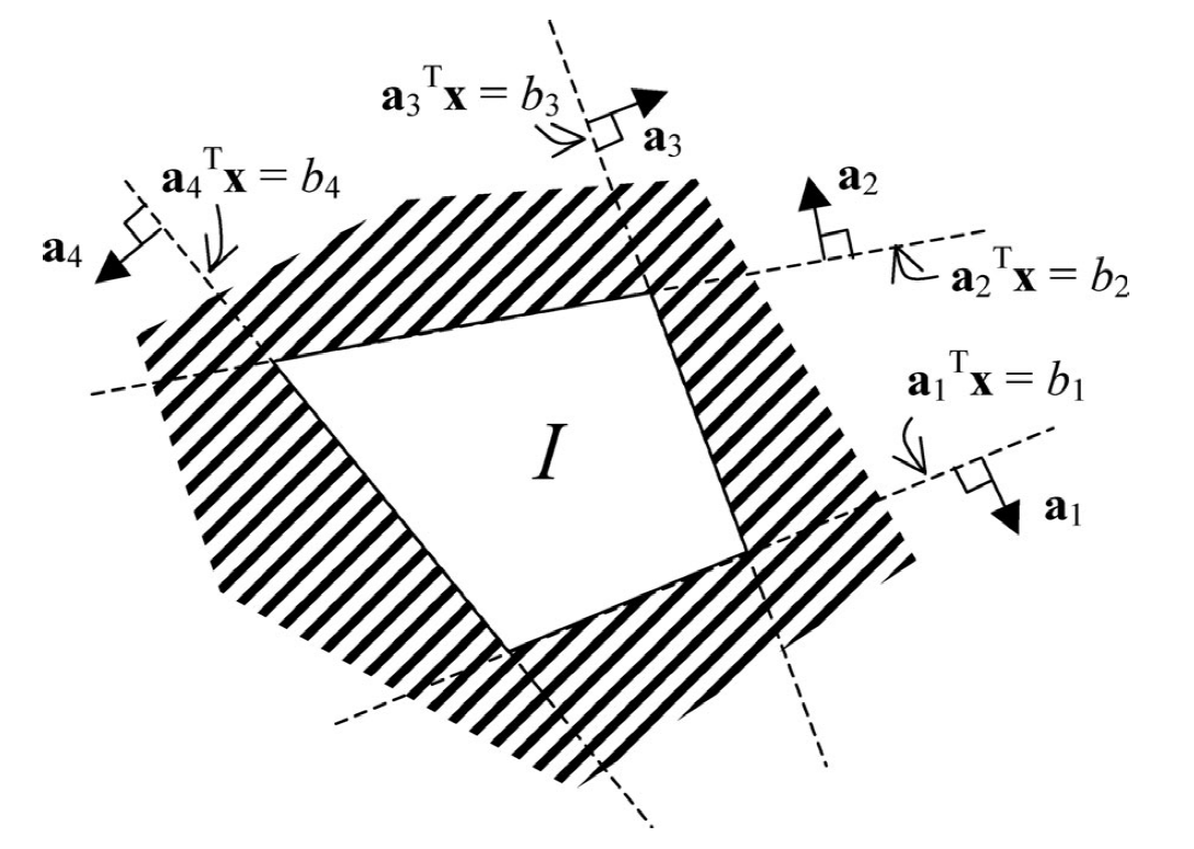
polygonal convex stay-in regions $\mathcal{I}$: states much remain
$$
\mathcal{I} \Longleftrightarrow \bigwedge_{t \in T(\mathcal{I})} \bigwedge_{i \in G(\mathcal{I})} \mathbf{a}{i}^{\prime} \mathbf{x}{t} \leq b_{i}
$$Polygonal convex obstacles: outside of which state must remain.
$$
\mathcal{O} \Longleftrightarrow \bigwedge_{t \in T(\mathcal{O})} \bigvee_{i \in G(\mathcal{O})} \mathbf{a}{i}^{\prime} \mathbf{x}{t} \geq b_{i}
$$
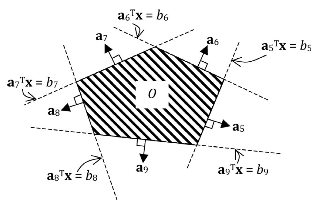
Note that nonconvex obstacles can be created by composing several convex obstacles.
Problem formulation:
Problem 1: Chance-constrained path-planning problem:
$$
\begin{array}=
&{\min\limits_{\mathbf{u}{0}, \ldots, \mathbf{u}{k-1}} g\left(\mathbf{u}{0}, \ldots, \mathbf{u}{k-1}, \overline{\mathbf{x}}{0}, \ldots, \overline{\mathbf{x}}{k}\right)} \ {\text{subject to: }} \
&{\overline{\mathbf{x}}{k}=\mathbf{x}{\mathrm{goal}}} \
&{\mathbf{x}{t+1}=A \mathbf{x}{t}+B \mathbf{u}{t}+\omega{t}} \
&{\mathbf{x}{0} \sim \mathcal{N}\left(\hat{\mathbf{x}}{0}, P_{0}\right) \omega_{t} \sim \mathcal{N}(0, Q)} \
&{P \left( \left(\bigwedge_{i=1}^{N_{\mathcal{I}}} \mathcal{I}{i}\right) \wedge \left(\bigwedge{j=1}^{N_{O}} \mathcal{O}{j}\right) \right) \geq 1-\Delta}
\end{array}
$$
where $g(\cdot)$ is a piecewise linear cost function, $N{\mathcal{I}}$ and $N_{\mathcal{O}}$ are number of stay-in regions and obstacles. $\overline{\mathbb{x}}$ means the expectation of $\mathbb{x}$.
Difficulty of solving:
- evaluating the chance constraint requires the computation of the integral of a multivariable Gaussian distribution over a finite, nonconvex region. This cannot be carried out in the closed form, and approximate techniques such as sampling are time consuming and introduce approximation error.
- even if this integral could be computed efficiently, its value is nonconvex in the decision variables due to the disjunctions in $\mathcal{O}_i$ . $\longrightarrow$ the resulting optimization problem is intractable. A typical approach to dealing with nonconvex feasible spaces is the branch-and-bound method, which decomposes a nonconvex problem into a tree of convex problems. However, the branch-and-bound method cannot be directly applied, since the nonconvex chance constraint cannot be decomposed trivially into subproblems.
Preliminary:
Disjunctive convex programs:
$$
\begin{aligned}
&{\min {X} h(X)} \
{\text { subject to : }} \
&{f{\text {eq }}(X)=0} \
&{\bigwedge_{i=1}^{n_{\text {dis }}} \bigvee_{j=1}^{n_{c l}} c_{i j}(X) \leq 0}
\end{aligned}
$$
where $c_{ij}(X)$ are convex function of $X$. $n_{\text{dis}}$ and $n_{\text{cl}}$ are the number of disjunctions and clauses within each disjunction.
Disjunctive linear program:
Same as above, but the $f_{\text{eq}}(X)$ and $c_{ij}(X)$ are linear function of $X$.
Difficulty of disjunctive convex program:
disjunction render the feasible region nonconvex. Nonconvex programs are intractable.
Method:
- Decompose the problem into a finite number of convex subproblems. The number of convex subproblems is exponential in the number of disjunctions $n_{\text{dis}}$. Brach-and-bound can find the global optimal solution while solving only small subset.
Propogation
initial state: Gaussian $\mathcal{N}(\hat{\mathbb{x}}0, P_0)$ + dynamics : linear + noise: Gaussian $\longrightarrow$ future state is Gaussian
$$
\begin{aligned}
p(X_t|\mathbb{u}{0,\cdots,k-1}) &\sim \mathcal{N}(\mu_t,\Sigma_t)\
\mu_t & =\sum\limits_{i=0}^{t-1}A^{t-i-1}B\mathbb{u}_i + A^t \hat{\mathbb{x}}0 \quad {\text{linear equation}}\
\sum_t &= \sum\limits{t=0}^{t-1} A^iQ(A^T)^i + A^tP_0(A^T)^t \quad {\text{not about control inputs}}
\end{aligned}
$$
Linear Chance Constraints as Deterministic Linear Constraints
Gaussian distribution:
pdf: $f(x|\mu,\sigma^2)=\frac{1}{\sqrt{2\pi \sigma^2}}e^{-\frac{(x-\mu)^2}{2\sigma^2}}$
cdf: $\Phi(x) = \frac{1}{\sqrt{2\pi}} \int\limits_{-\inf}^x e^{- \frac{t^2}{2}} dt$
erf: $\operatorname{erf}(x) = \frac{2}{\sqrt{\pi}} \int\limits_0^x e^{-t^2} dt$ (gives the probability of a random variable with normal distribution of mean 0 and variance 1/2 falling in the range $[-x,x]$)
Gaussian form translation: $f(x|\mu,\sigma^2)=\frac{1}{\sigma} \varphi(\frac{x-\mu}{\sigma})$