0%

3. Convex Analysis

3.1 Prove convex set:

  1. $x,y\in C$, then prove $\lambda x + (1-\lambda y) \in C$
  2. intersection of convex sets are convex
  3. $f$ is convex $\iff$ epigraph set is convex $f(x)\le \alpha$

3.2 Prove convex function:

  1. Prove $f(\lambda x + (1-\lambda)y) \le \lambda f(x) + (1-\lambda) y$
  2. (sum of) linear combination of convex function is convex
  3. $h$ convex, $g$ non-decreasing convex, $g\circ h$ is convex
  4. epigraph set is convex $f(x)\le \alpha$ $\iff$ $f$ is convex
  5. convex, then $x=\sum_{k=1}^k \lambda_jx^{j}$, where $\sum_{j=1}^k \lambda_j =1$, we have $f(x)\le \sum_{k=1}^k \lambda_j f(x^j)$ Jensen’s inequality:
  6. convex $\iff$ $f(y) \le f(x)+\nabla f(x)^T (y-x)$ Tangent plane characterization:
  7. convex $\iff$ $\langle \nabla f(\mathbb y)-\nabla f(\mathbb x), \mathbb y - \mathbb x \rangle \ge 0, \quad \forall \mathbb x, \mathbb y \in S$ monotone gradient condition
  8. convex $\iff$ Hessian is positive semidefinite

For constrained convex programming $\min{f(x)|x\in C}$, $x^*$ is global minimizer $\iff$ $\langle \triangledown f(x^*), x-x^* \rangle > 0, \forall x \in C$.

3.3 Projection: $\Pi_C(z) = \mathrm{argmin} { \frac{1}{2} |x-z|^2 \vert x\in C }$

  • $x^* = \Pi_C(z)$ $\iff$ $\langle z-x^*, x-x^* \rangle \leq 0, \forall x\in C$
  • $| \Pi_C(z) - \Pi_C(w) | \leq |z-w |$.
  • C is linear subspace, $z-x^*\perp C$, then $z = \Pi_C(z) + (z-\Pi_C(z)), \quad \text{and } \quad \langle z-\Pi_C(z), \Pi_C(z)\rangle = 0$
  • C is closed convex cone, $\langle z-\Pi_C(z), \Pi_C(z)\rangle = 0$
  • If $\theta (x) = \frac{1}{2} | x-\Pi_C(x)|^2$, then $\theta(\cdot)$ is a continuously differentiable convex function and $\nabla \theta(x) = x-\Pi_C(x)$

3.4 Cones:

  • Dual cone: $S^* = { y\in S | \langle x,y \rangle \ge 0, \forall x\in S }$. Self-dual cone $C^*=C$, including $\mathbb S_+^n$, $\mathbb R^n$,
  • Polar cone: $S^\circ = -S^*$
  • $(C^*)^*=C$.
  • Spectral cone $\mathcal K^*$, Nuclear-norm cone $\mathcal C$, $\mathrm {COP}_n$, $\mathrm {CPP}_n$, double nonnegative cone $\mathbb D_n$. [Chapter 3, P79]
  • $z-\Pi_C(z) = \Pi_{C^\circ}(z)$, if $C$ is closed convex cone.
  • Normal cone:
    • $N_C(\bar x) = {z\in \mathcal E | \langle z, x-\bar x \rangle \leq 0, \forall x\in C}$ where $\bar x \in C$.
    • $u\in N_C(y) \iff y=\Pi_C(y+u)$
    • $N_{C_1} (\bar x) + N_{C_2} (\bar x) \subset N_{C_1\cap C_2} (\bar x)$ where $\bar x \in C_1 \cap C_2$.
    • $C=\mathcal S^n_+$. $X=U_1D_1U_1^T, D_1 = \mathrm{diag}(d_1, \cdots, d_r)$ with descending order. $N_C(X)={-U_2\Delta U_2^T}$. [P81]

3.5 Subgradient:

  • $\langle v-u, y-x \rangle \ge 0, \quad \forall u\in \part f(x), v\in \part f(y)$ Monotone mapping

  • $\part \delta_C(x) = \begin{cases}
    \empty \quad & \text{if }x\notin C \
    \mathcal N_C(x)= \text{normal cone of $C$ at $x$} \quad & \text{if }x\in C
    \end{cases}$ where $C$ is convex subset of $\mathbb R^n$

  • $\part f(0) = { y\in \mathbb R^n | |y|_\infty \le 1 }$, if $f(x) = | x |_1$ [P85]

3.6 Frenchel Conjugate:

$$
f^*(y) = \sup { \langle y,x \rangle - f(x) | x\in \mathcal E }, y\in \mathcal \ E
$$

  • $f^*$ is always closed and convex, even if $f$ is non-convex or not closed.

  • Equivalent condition

    1. $f(x) + f^*(x^*) = \langle x, x^* \rangle$
    2. $x^* \in \part f(x)$
    3. $x \in \part f^*(x^*)$
    4. $\langle x, x^* \rangle - f(x) =\max_{z\in \mathcal E} {\langle z, x^* \rangle - f(z)}$
    5. $\langle x, x^* \rangle - f^*(x^*) =\max_{z^\in \mathcal E} {\langle x, z^ \rangle - f^*(z^*)}$
    6. $(f^*)^* = f$

3.7 Moreau-Yosida regularization and proximal mapping

$$
\begin{array}{ll}{\text { MY regularization of } f \text { at } x:} & {M_{f}(x)=\min {y \in \mathcal{E}}\left{\phi(y ; x):=f(y)+\frac{1}{2}|y-x|^{2}\right}} \ {\text { Proximal mapping } f \text { at } x:} & {P{f}(x)=\operatorname{argmin}_{y \in \mathcal{E}}{\phi(y ; x):=f(y)+\frac{1}{2}|y-x|^{2}}}\end{array}
$$

  • $x=P_f(x)+P_{f^*}(x), \forall x\in \mathcal E$
  • $f(x)=\lambda |x|_1$, $f^*(z)=\delta_C(z)$ where $C=\part f(0)={z\in \mathbb R^n | |z|_\infty \le \lambda }$ [P91]
  • If $f=\delta_C$, $P_{\delta_{C}}(x)=\operatorname{argmin}{y \in \mathcal{E}}\left{\delta{C}(y)+\frac{1}{2}|y-x|\right}=\operatorname{argmin}{y \in C} \frac{1}{2}|y-x|^{2}=\Pi{C}(x)$. [P92]
  • if $C=\mathbb S_+^n$, Then $\Pi_C(x)=Q\mathrm{diag}d_+ Q^T \quad \text{using spectral decomposition } x=Q \mathrm{diag}dQ^T$

4. Gradient Methods

Descent direction: direction $\mathbf d$ such that $\langle \nabla f(x^*), d\rangle <0 $.

Steepest decent direction: direction $\mathbf d$ such that $\mathbf d^* = - \nabla f(x^*)$.

  1. Steepest descent method with exact line search: + Convergence rate

  2. Accelerated Proximal Gradient method: + Error, complexity

    1. Sparse regression [P112]
    2. Projection on to convex cone $\mathrm{DNN}n^* = \mathbb S+^n + \mathcal N^n$ [P112]
  3. Gradient Projection Method:

    $x^{k+1} = P_Q(x^k - \alpha_k \nabla f(x^k))$, where $x(\alpha) = x-\alpha \nabla f(x)$, $x_Q(\alpha) = P_!(x(\alpha))$

  4. Stochastic Gradient Descent Method

5. Basic NLP (KKT)

(LICQ): Linear Independency Constraint Qualification : regular point : $\nabla h_i$ and $\nabla g_i$ are linear independent.

KKT necessary condition:

  • 1st order:

    $\begin{array}{l}{[1] \quad \nabla f\left(\mathrm{x}^{}\right)+\sum_{i=1}^{m} \lambda_{i}^{} \nabla g_{i}\left(\mathrm{x}^{}\right)+\sum_{j=1}^{p} \mu_{j}^{} \nabla h_{j}\left(\mathrm{x}^{}\right)=0} \ {[2] \quad g_{i}\left(\mathrm{x}^{}\right)=0, \quad \forall i=1,2, \cdots, m} \ {[3] \quad \mu_{j}^{} \geq 0, h_{j}\left(\mathrm{x}^{}\right) \leq 0, \quad \mu_{j}^{} h_{j}\left(\mathrm{x}^{}\right)=0, \quad \forall j=1,2, \cdots, p}\end{array}$

  • 2nd order: $y^T H_L(x^*) y \ge 0$ where $y\in T(x^*)$ tangent plane

    • Easier check: $Z(x^*)H_L(x^*)Z(x^*)$ is positive semidefinite

Steps:

  1. Check regularity condition
  2. verify KKT first order necessary condition.
  3. verify KKT second order necessary condition
    1. Hessian matrix
    2. basis of null space of $\mathcal D(\mathbb x^*)^T$
    3. definiteness check

Projection onto simplex: [P139-140]

relax multipliers

KKT sufficient conditions: 1st + 2nd

steps:

  1. verify it’s KKT point.
  2. verify it satisfy the second order sufficient condition
    1. Hessian matrix
    2. $Z(\mathbf x^*)$
    3. Determine definiteness

Important points:

  1. KKT point is an optimal solution under convexity, but a global minimizer of a convex program may not be a KKT point.

  2. With regularity condition, a global minimizer is a KKT point. For convex programming problem with at least one inequality constraints, the Slater’s condition ensures that a global minimizer is a KKT point.

    slater’s condition: there exists $\hat{\mathbb x} ∈ \mathbb R^n$ such that $g_i(\hat{\mathbb x}) = 0, ∀ i = 1,\cdots, m$ and $h_j(\hat{\mathbb x}) < 0, ∀ j = 1, . . . , p$.

     Slater's condition states that the feasible region must have an [interior point](https://en.wikipedia.org/wiki/Interior_(topology)).
    
  3. Linear equality constrained problem:

    a point $x^∗ ∈ S$ is a KKT point $\iff$ $x^∗$ is a global minimizer of $f$ on $S$.

    No regularity or slater condition is needed.

  4. LInear + convex quadratic programming.

6. Lagrangian duality

optimal value of dual problem is smaller than optimal value of primal problem. Duality gap;

Saddle point optimality $\longleftrightarrow$ KKT

  1. For a fixed $\mathbb x^∗$, $(λ^∗, μ^∗)$ maximizes $L(\mathbb x^∗, λ, μ)$ over all $(λ, μ)$ with $μ ≥ 0$.
  2. For a fixed $(λ^∗, μ^∗)$ , $\mathbb{x}^*$ minimizes $L(\mathbb x, λ^∗, μ^∗)$ over all $x ∈ X$.
  3. saddle point $(\mathbb x^*, \lambda^*,\mu^*)$ $\Rightarrow$ KKT condition. but inverse is not true in general.
  4. KKT point of a convex program is a saddle point.

7. Nonlinear conic programming

Sparse regression problem:

  • objective function is convex

  • APG: [P112]

  • KKT: [P153-154]

  1. Chapter 7. conic programming

  2. Chapter 8. sPADMM

    P214

Indicator function:

  • Indicator function: $\delta_C(x) = \begin{cases} 0, & x\in C \ \infty, & x\notin C \end{cases}$

$$
\delta_{S_+^n}^* = \delta_{-S_+^n}
$$

$$
\mathrm{Prof}_f(x) = (I+\lambda \part f)^{-1}
$$

$P_f(x) = x-P_{f^*}(x)$

Proximal $P_f$ and Projection $\Pi_C(f(x))$ : When $f=\delta$ indicator function, the two operator are equivalent.

$f(x) = \lambda |x|_1 $, then $f^*(z) = \delta_C(z)$ where $C=\part f(0) = {z\in\mathbb R^n | |z|_\infty \le \lambda }$, the proximal function $P_f(x) = \mathrm {sgn} (x) \circ \max{|x|-\lambda }$ [P91-92]

$f=\delta_C$, $C$ is closed and convex, the proximal and projection operator are equivalent, because $P_{\delta_{C}}(x)=\operatorname{argmin}{y \in \mathcal{E}}\left{\delta{C}(y)+\frac{1}{2}|y-x|\right}=\operatorname{argmin}{y \in C} \frac{1}{2}|y-x|^{2}=\Pi{C}(x)$. When $C=\mathbb S_+^n$, then $\Pi_C(x)=Q \mathrm {diag}(d_+) Q^T$ using spectral decomposition $x=Q\mathrm {diag}(d) Q^T$

$f(x)=|x|_*$, then the $P_f(x) = V\Sigma^+ U^T$.

$x^* = P_f(x^*)$ will converge to the optimum of $f$, i.e., $x^*$.

Dual norm: [P88]

  • $f(x)=\lambda |x|1$, then $f^*(x) = \delta{B_\lambda}$, where $B_\lambda = {x\in \mathbb R^n | |x|_\infty\leq \lambda}$.
  • $f(x)=\lambda |x|\infty$, then $f^*(x) = \delta{B_\lambda}$, where $B_\lambda = {x\in \mathbb R^n | |x|_1\leq \lambda}$.
  • $f(x)=\lambda |x|m$, then $f^*(x) = \delta{B_\lambda}$, where $B_\lambda = {x\in \mathbb R^n | |x|_n\leq \lambda}$, $\frac{1}{m}+\frac{1}{n}=1$, called dual norm.
  • $\ell_2$ norm is self-dual norm.

$y\in N_C(x)$, then $y\in \Pi_C(x+y)$

$x=P_f(x)+P_{f^*}(x), \forall x\in \mathcal E$

$G = \Pi_{\mathbb S_+^*}(G) - \Pi_{\mathbb S_+^n}(-G)$

$\min{ \frac{1}{2}|G+Z|^2 | Z\in \mathbb S_+^n} = \frac{1}{2} | G+\Pi_{\mathbb S^n_+}(G)|^2 = \frac{1}{2} |\Pi_{\mathbb S_+^n}(G) |^2$

  1. $\mathbb x \in S \iff \mathbb x = \mathbb x^* + \mathbb z$ for some $\mathbb z \in \operatorname{Null}(A)$. 【space of x】
  2. $\mathbb y^T \mathbb z = 0$, $\forall \mathbb z \in \operatorname{Null}(\mathbf A) \iff \exist \lambda^* \in \mathbb R^m$ s.t. $\mathbb y+ \mathbf A^T \lambda^*=0$.

The linear map $\mathcal A(X) = \begin{bmatrix} \langle A_1, X \rangle \ \vdots \ \langle A_m, X \rangle \end{bmatrix}$. Let $\mathcal A^* $ be adjoint of $\mathcal A$ as $\mathcal A^* y = \sum\limits_{k=1}^m y_kA_k, y\in \mathbb R^m$.
$$
\langle \mathcal A^* y, X \rangle = \langle y, \mathcal A X \rangle
$$
if $\mathcal A(X) = \operatorname{diag} (X)$, then $A_k = E_{kk}$, and $\mathcal A^* y = \operatorname{diag} (y)$.

Dual problems:

  • Linear programs + dual problem:

  • Quadratic program + dual problem

  • Square function + Linear inequality constraints [P177]

  • NLP + dual problem [P178,180]

  • SDP + Dual Problem [P178, P180]

  • SDPLS + dual problem [P179, ]

  • Quadratic Semidefinite problem + Dual problem

  • Convex quadratic composite optimization problem + dual problem:

  • d

in general, Hessian $H_f(\mathbb x)$ is not symmetric. But, if $f$ has continuous second order derivatives, then the Hessian matrix $H_f( \mathbb x)$ is symmetric.

Positive semidefinite: if $\mathbb x^T \mathbf A \mathbb x \ge 0, \forall \mathbb x \in \mathbb R^n$.

positive definite: if $\mathbb x^T \mathbf A \mathbb x \ge 0, \forall \mathbb x \neq 0$.

if $\mathbf A$ is a real symmetric $n\times n$ matrix.

  • if $\mathbf A$ is positive semidefinite $\iff$ every eigenvalue of $A$ is nonnegative $\lambda > 0$.
  • $\lambda_{\min} (\mathbf A) | \mathbb x |^2 \leq \langle \mathbb x, \mathbf A \mathbb x\rangle \leq \lambda_{\max} (\mathbf A) |\mathbb x |^2, \ \forall \mathbb x \in \mathbb R^{n\times n}$

Inner product of matrix:

  • $A,B \in \mathbb R^{m\times n}$, have $\langle A,B \rangle = \sum\limits_{i=1}^{m} \sum\limits_{j=1}^{n} A_{ij} B_{ij} = \operatorname{Tr}(A^TB)$

Frobenius norm:

  • $|A|F = \sqrt{ \sum\limits{i=1}^{m} \sum\limits_{j=1}^{n} |A_{ij}|^2} = \sqrt{\operatorname{Tr}(A^TA)}$

Sherman-Morrison-Woodbury (SMW) formula

Suppose $U,V \in \mathbb R^{n\times p}$ and $| UV^T | <1$, Then
$$
(I+UV^T)^{-1} = I-UG^{-1} V^T \quad \in \mathbb R^{n\times n}
$$
where $G=I_p + V^TU \in \mathbb R^{p\times p}$

When $n$ is large, it’s hard to compute the inverse of $(I+UV^T)$. But if using the SMW formula, it’s easy to compute by transforming it as $I-UG^{-1} V^T$, because the inverse of $G$ is easy to compute ($p$ is small).

If $(I+UV^T)$ is nonsingular, than the SMW formula $(I+UV^T)^{-1} = I-UG^{-1} V^T$holds without requiring $| UV^T | <1$

Bounded: $|\mathbb x | \leq M, \forall \mathbb x \in S$. If $C_1, C_2$ are bounded, then $C_1 \cup C_2$ is bounded.

Closed: $\lim\limits_{n\rightarrow \infin} \mathbb x_n \in S$. If $C_1, C_2$ are closed, then $C_1\cap C_2$ is closed.

Prove method: if function $g$ is continuous, then set $S={\mathbb x\in \mathbb R^n | g(\mathbb x) \le 0}$ is closed. Or $S={\mathbb x\in \mathbb R^n | g(\mathbb x) \ge 0}$ is closed. Or $S={\mathbb x\in \mathbb R^n | g(\mathbb x) = 0}$ is closed.

Example:

Prove $C = \left{ \begin{pmatrix} x \ x^2 \end{pmatrix} \in \mathbb R^2 \right}$ is closed.

Solution:
$$
C = \left{ \begin{pmatrix} x \ x^2 \end{pmatrix} \in \mathbb R^2 \right} = \left{ \begin{pmatrix} x_1 \ x_2 \end{pmatrix} \in \mathbb R^2 \quad \vert \quad g(\mathbb x) := x_2-x_1^2 = 0 \right}.
$$
since $g$ is continuous, so $C$ is closed.

Compactness: Closed + Bounded

Coercive function:
$$
\lim\limits_{|\mathbb x| \rightarrow \infty} f(\mathbb x) = +\infty
$$
Which means that the function value $f(\mathbb x)$ will increase without bound as $\mathbb x$ moves away from the origin in all possible directions.

==Existence of optimal solution:==

  1. a continuous function $g:\mathbb R^n \rightarrow \mathbb R$ on a nonempty closed and bounded set $S \subset \mathbb R^n$ has a global maximum and a global minimum point in $S$.

  2. $f:\mathbb R^n \rightarrow \mathbb R$ is continuous function. If $f$ is coercive, then $f$ has at least one global minimizer. (when x is not bounded)

A stationary point $\mathbb x^*$ with $H_f(\mathbb x^*)$ positive semi-definite, the status of $\mathbb x^*$ can only be determined by analyzing $f(\mathbb x^*)$ is a neighborhood of $\mathbb x^*$. Can obtain a global minimizer by comparing the objective value at the stationary points.

4.1 Unconstrained Optimization

Descent direction: direction $\mathbf d$ such that $\langle \nabla f(x^*), d\rangle <0 $.

Steepest decent direction: direction $\mathbf d$ such that $\mathbf d^* = - \nabla f(x^*)$.

Steepest descent method with exact line search:

[step 0]

[step k]

steepest descent method follows a zig-zag path towards $\mathbf x^*$ with the right angle at each turn. $\longrightarrow$ slow

Theorem:

Steepest descent method with exact line search moves in perpendicular steps. More precisely, if $\mathbf x^{(k)}$ is a steepest descent sequence for a function $f(\mathbf x)$, then for each $k$, the vector joining $\mathbf x^{(k)}$ to $\mathbf x^{(k+1)}$ (i.e. $\mathbf x^{(k+1)} - \mathbf x^{(k)}$) is orthogonal (perpendicular) to the vector joining $\mathbf x^{(k+1)}$ to $\mathbf x^{(k+2)}$ (i.e. $\mathbf x^{(k+2)}-\mathbf x^{(k+1)}$).

Property:

  • monotonic decreasing property
  • convergence
    • limit of any convergent subsequence of ${\mathbf x^{(k)}}$ is a critical point of $f(\mathbf x)$.

4.1.1 convergence rate for unconstrained quadratic minimization

$$
\min_{\mathbf x\in \mathbb R^n} q(\mathbf x)=\frac{1}{2}\mathbf x^T \mathbf Q \mathbf x
$$

Proposition:

$\mathbf Q$ is symmetric and positive definite, use steepest descent method with exact line search,

  1. Let $\mathbf d^k = \nabla q(\mathbf x^k)=\mathbf Q \mathbf x^k$.
    $$
    \frac{q\left(\mathrm{x}^{k+1}\right)}{q\left(\mathrm{x}^{k}\right)}= 1-\frac{\left\langle\mathrm{d}^{k}, \mathrm{d}^{k}\right\rangle^{2}}{\left\langle\mathrm{d}^{k}, \mathrm{Qd}^{k}\right\rangle\left\langle\mathrm{d}^{k}, \mathrm{Q}^{-1} \mathrm{d}^{k}\right\rangle}
    $$

  2. $$
    \frac{q\left(\mathrm{x}^{(k+1)}\right)}{q\left(\mathrm{x}^{(k)}\right)} \leq\left[\frac{\kappa(\mathrm{Q})-1}{\kappa(\mathrm{Q})+1}\right]^{2}=: \rho(\mathrm{Q})
    $$

    where $\kappa(\mathrm{Q})=\lambda_n / \lambda_1$, $\lambda_n, \lambda_1$ are the largest and smallest eigenvalues of $\mathbf Q$.

Remark.

  • the convergence rate $\rho(\mathbf Q)$ depends on $\kappa(\mathbf Q)$. When $\kappa(\mathbf Q)$ is large, the convergence rate
    $$
    \rho(\mathbf Q) \approx 1-\frac{4}{\kappa(\mathbf Q)}
    $$

  • In $\mathbb R^2$, the contours of $q(\mathbf x)$ are ellipses. And $\kappa(\mathbf Q)$ is the ratio between the length of the principal axes of the ellipses. Thus the larger the value of $\kappa(\mathbf Q)$, the more elongated the ellipses are.

  • The number of iterations needed to reduce the relative error $q(\mathbf x^k)/q(\mathbf x^0)$ to smaller than $\epsilon$ is given by
    $$
    k=\left[ \frac{\log \epsilon}{\log \rho(\mathbf Q)} \right] + 1
    $$
    where $[a]$ denotes the largest integer less than or equal to $a$.

4.1.2 Convergence rate for strongly convex function

$f$: strongly convex with parameter $m$ and has $M$-Lipschitz continuous gradient. Its Hessian:
$$
mI \preceq H_f (\mathbf x) \preceq MI, \forall \mathbf x\in S
$$
Lemma:

$\mathbf x^*$ is minimizer of $\min{f(\mathbf x)| \mathbf x \in S}$. Then
$$
f(\mathrm{x})-\frac{1}{2 m}|\nabla f(\mathrm{x})|^{2} \leq f\left(\mathrm{x}^{*}\right) \leq f(\mathrm{x})-\frac{1}{2 M}|\nabla f(\mathrm{x})|^{2} \quad \forall \mathrm{x} \in S
$$
Theorem:

Let $\mathbf x^*$ be unique minimizer. $E_k = f(\mathbf x^k) - f(\mathbf x^*)$. Then
$$
\begin{aligned} E_{k+1} & \leq E_{k}-\frac{1}{2 M}\left|\nabla f\left(\mathrm{x}^{k}\right)\right|^{2} \quad \text { (descent inequality) } \ E_{k+1} & \leq E_{k}\left(1-\frac{m}{M}\right) \end{aligned}
$$
Remark:

based on this theorem, we have
$$
{\qquad E\left(\mathrm{x}^{k+1}\right) / E\left(\mathrm{x}^{1}\right) \leq(1-m / M)^{k} \leq \varepsilon}
$$
implies that we need the number of iterations $k$ to satisfy
$$
{\left.\qquad k \geq \frac{\log \varepsilon^{-1}}{\log \rho^{-1}} \approx \frac{m}{M} \log \varepsilon^{-1} \quad \text { (if } m / M \ll 1\right)}
$$
where $\rho = 1-m/M$.

4.2Line search strategies

  1. minimization rule = exact line search
  2. Armijo rule
  3. nonmonotone line search
  4. monotone line search , BB stepsize

4.3 Accelerated proximal gradient

smooth convex function $f$ with $L$-Lipstchitz continuous gradient
$$
\min { F(x):= f(x)+g(x) | x\in \mathbb R^n }
$$
$g$ is proper closed convex function (maybe non-differentiable).

Problem:
$$
\hat x = \mathrm{argmin} {g(x)+q(x;\bar x) | x\in \mathbb R^n }
$$
where $q(x;\bar x) = f(\bar x) + \langle \nabla f(\bar x), x-\bar x\rangle + \frac{1}{2} \langle x-\bar x, H(x-\bar x) \rangle $.

APG method

[step 1]

[step 2]

Lemma:

Assume $f(\hat x) \le q(\hat x; \bar x)$. The descent property:
$$
F(x)+\frac{1}{2}|x-\bar{x}|{H}^{2} \geq F(\hat{x})+\frac{1}{2}|x-\hat{x}|{H}^{2} \quad \forall x \in \mathbb{R}^{n}
$$
(the assumption $\Longrightarrow$ 1-Lipschitz continuous )

Theorem

Error

complexity

Two for PG and APG

example:

  1. Sparse regression problem $\min{\frac{1}{2} |Ax-b|^2 + \rho|x|_1 | x\in \mathbb R^n }$. Let $f(x) = \frac{1}{2} |Ax-b|^2$ and $g(x) = \rho|x|1$. $\nabla f(x) = A^T(Ax-b)$ is Lipschitz continuous with modulus $L=\lambda{\max}(AA^T)$. Let $H=LI_n$, the APG method subproblem is given by
    $$
    x^{k+1}=\operatorname{argmin}\left{g(x)+\left\langle\nabla f\left(\bar{x}^{k}\right), x-\bar{x}^{k}\right\rangle+\frac{L}{2}\left|x-\bar{x}^{k}\right|^{2} | x \in \mathbb{R}^{n}\right}
    $$

  2. given $G\in \mathbb S^n$. Projection onto the closed convex cone $\mathrm{DNN}n^* = \mathbb S+^n + \mathcal N^n$:
    $$
    \begin{array}{l}{\min \left{\frac{1}{2}|S+Z-G|^{2} | S \in \mathbb{S}{+}^{n}, Z \in \mathcal{N}^n \right} }\ {=\min \left{\frac{1}{2}\left|\Pi{\mathcal{N}^{n}}(S-G)\right|^{2} | S \in \mathbb{S}{+}^{n}\right}} \ {=\min \left{f(S)+\delta{\mathrm{S}{+}^{n}}(S) | S \in \mathbb{S}^{n}\right}}\end{array}
    $$
    where $f(S)=\frac{1}{2} | \Pi
    {\mathcal N^n} (S-G) |^2$. The optimality condition for a minimizer $\bar S$ of the last minimization problem is given as follows:
    $$
    \begin{array}{l}{0 \in \partial\left(f+\delta_{\mathrm{S}{+}^{n}}\right)(\bar{S})=\partial f(\bar{S})+\partial \delta{\mathrm{S}{+}}^{\mathrm{n}}(\bar{S})} \ {\Leftrightarrow-\nabla f(\bar{S}) \in \partial \delta{\mathrm{S}{+}}^{n}(\bar{S})} \ {\Leftrightarrow-\nabla f(\bar{S}) \in\left(I+\partial \delta{\mathrm{S}{+}}\right)(\bar{S})} \ {\Leftrightarrow \bar{S}=\left(I+\partial \delta{\mathrm{S}{+}}\right)^{-1}(\bar{S}-\nabla f(\bar{S}))=\Pi{\mathrm{S}{+}^{n}}(\bar{S}-\nabla f(\bar{S}))} \
    \end{array}
    $$
    we have $\nabla f(S) = \Pi
    {mathcal N^n}(S-G)$, and
    $$
    {\begin{aligned}|\nabla f(S)-\nabla f(S)| &=\left|\Pi_{N^{n}}(S-G)-\Pi_{\mathcal{N}^{n}}\left(S^{\prime}-G\right)\right| \ & \leq\left|(S-G)-\left(S^{\prime}-G\right)\right|=\left|S-S^{\prime}\right| \end{aligned}}
    $$
    Thus $∇f(·)$ is Lipschitz continuous with modulus $L = 1$. Pick $H = LI_n$, the APG subproblem is given by
    $$
    \begin{aligned} S^{k+1} &=\operatorname{argmin}\left{\delta_{\mathrm{S}{+}^{n}}(S)+\left\langle\nabla f\left(\bar{S}^{k}\right), S-\bar{S}^{k}\right\rangle+\frac{1}{2}\left|S-\bar{S}^{k}\right|^{2} | S \in \mathbb{S}^{n}\right} \ &=\operatorname{argmin}\left{\frac{1}{2}\left|S-\bar{S}^{k}+\nabla f\left(\bar{S}^{k}\right)\right|^{2} | S \in \mathbb{S}{+}^{n}\right} \ &=\prod_{\mathrm{S}_{+}^{n}}\left(\bar{S}^{k}-\nabla f\left(\bar{S}^{k}\right)\right) \end{aligned}
    $$
    Observe that the subproblem is like carrying out a fixed-point iteration on the optimality condition.

Karush-Kuhn-Tucker (KKT) necessary conditions for local minimizers that generalize the Lagrange Multiplier Method. The KKT necessary conditions are useful in locating possible candidates for a global minimizer.

Constraint qualification

  • Active constraints

  • Regular point :

    $x^*$ be feasible point of NLP, Let $J(x^*) = \left{ j\in {1, \cdots, p} : h_j(x^*)=0 \right}$ be index set of active constraints at $x^*$. The set of gradient vectors
    $$
    { \nabla g_i(x^*) : i=1, 2, \cdots, m } \cup {\nabla h_j(x^*) : j\in J(x^*) }
    $$
    is linearly independent. $x^*$ is regular point.

Linearly Independence Constraint Qualification (LICQ)

  • check whether linear independence, check whether the matrix of all gradient vector of active constraints is full rank.

5.1 KKT necessary conditions

We state the Karush-Kuhn-Tucker necessary conditions for a local minimizer $x^∗$ at which the regularity condition holds

5.1.1 KKT first order necessary conditions:

$$
\begin{aligned} \nabla f\left(\mathrm{x}^{}\right)+\sum_{i=1}^{m} \lambda_{i}^{} \nabla g_{i}\left(\mathrm{x}^{}\right)+\sum_{j=1}^{p} \mu_{j}^{} \nabla h_{j}\left(\mathrm{x}^{}\right) = 0 \ \mu_{j}^{} \geq 0, &\ \forall j=1,2, \cdots, p \ \mu_{j}^{}=0, & \ \forall j \notin J\left(\mathrm{x}^{}\right) \end{aligned}
$$

  1. For NLP with no equality constraints, active constraint is only $h_1(x)\leq 0$. So, $\nabla f(x^*) + \mu_1^* \nabla h_1(x^*) = 0$,

    the direction of steep descent $-\nabla f(x^*)$ must be in same direction as $\nabla h_1(x^*)$ onward normal to boundary.

  2. For NLP with no equality constraints, only two active constraints, $\nabla f(x^*) + \mu_1^* \nabla h_1(x^*) + \mu_2^* \nabla h_2(x^*) = 0$.

    the direction of steep descent $-\nabla f(x^*)$ must lie in the cone spanned by the outward normals $\nabla h_1(x^*), \nabla h_2(x^*)$ to the boundaries $h_1(x)=0$ and $h_2(x)=0$.

  3. For NLP with no equality constraints, $x^*$ is interior of feasible region, $\nabla f(x^*)=0$, as unconstrained minimization problem.

5.1.2 KKT second order necessary condition:

$$
{\qquad H_{L}\left(\mathrm{x}^{}\right) :=H_{f}\left(\mathrm{x}^{}\right)+\sum_{i=1}^{m} \lambda_{i}^{} H_{g_{i}}\left(\mathrm{x}^{}\right)+\sum_{j=1}^{p} \mu_{j}^{} H_{h_{j}}\left(\mathrm{x}^{}\right)}
$$

If $\mathbb x^* $ is a local minimizer, then
$$
{\mathrm{y}^{T} H_{L}\left(\mathrm{x}^{}\right) \mathrm{y} \geq 0}
$$
for all $\mathbb y\in T(\mathbb x^
)$, where
$$
T(\mathbb x^*) = \left{ \mathbb y\in \mathbb{R}^n:
\begin{array}{}
\nabla g_{i}\left(\mathrm{x}^{}\right)^{T} \mathbf{y} = 0, i=1,2, \cdots, m \
\nabla h_{j}\left(\mathrm{x}^{
}\right)^{T} \mathrm{y} = 0, j \in J\left(\mathrm{x}^{*}\right)
\end{array} \right}
$$

in fact, $T(\mathbb x^*)$ is tangent plane

  1. set $T(x^*)$ consists of vectors in the tangent space to $S$ at $x^*$.

    Normal space $N(x^*)$ is subspace spanned by $\nabla g_1(x^*), \cdots, \nabla g_m (x^*), \nabla h_j(x^*), \forall j \in J(x^*)$.

    Tangent space $T(x^*) = { \mathbb y: \mathbb u^T \mathbb y = 0, \forall \mathbb u \in N(\mathbb x^*) }$.

  2. For NLP with no equality constraints, if $x^*$ is in interior of feasible region, $T(x^*) = \mathbb R^*$. 2nd KKT becomes $H_L(x^*) = H_f(x^*)$ must be positive semidefinite.

​ easier check for 2nd KKT.

​ matrix $\mathcal D(\mathbb x^*) = \left( \nabla g_1(\mathbb x^*), \cdots, \nabla g_m(\mathbb x^*), [\nabla h_j(\mathbb x^*) : j \in J(\mathbb x^*)] \right)$
$$
\mathbb y^T H_L(\mathbb x^*) \mathbb y \ge 0, \forall \mathbb y \in T(\mathbb x^*) \iff Z(\mathbb x^*)^T H_L(\mathbb x^*) Z(\mathbb x^*) \text{ is positive semidefinite}
$$
​ where $Z(\mathbb x^*)$ is a matrix whose columns forms a basis of the null space of $\mathcal D (\mathbb x^*)$. $T(x) = Z(x) u$

5.1.2 Steps:

  1. Check regularity condition
  2. verify KKT first order necessary condition.
  3. verify KKT second order necessary condition
    1. Hessian matrix
    2. basis of null space of $\mathcal D(\mathbb x^*)^T$
    3. definiteness check

Since the regularity condition for the KKT Theorem is not satisfied, the global minimizer $x^∗$ may not be found among the KKT points.

KKT necessary conditions can be used to find global minimizers.

==Corollary 2.3==

Suppose the following two conditions hold:

  1. a global minimizer $x^∗$ is known to exist for an NLP.
  2. $x^∗$ is a regular point.

Then $x^∗$ is a KKT point, i.e. there exists $λ^∗ ∈ \mathbb R^m$ and $μ^∗ ∈ \mathbb R^p$ such that the following conditions hold.
$$
\begin{array}{l}{[1] \quad \nabla f\left(\mathrm{x}^{}\right)+\sum_{i=1}^{m} \lambda_{i}^{} \nabla g_{i}\left(\mathrm{x}^{}\right)+\sum_{j=1}^{p} \mu_{j}^{} \nabla h_{j}\left(\mathrm{x}^{}\right)=0} \ {[2] \quad g_{i}\left(\mathrm{x}^{}\right)=0, \quad \forall i=1,2, \cdots, m} \ {[3] \quad \mu_{j}^{} \geq 0, h_{j}\left(\mathrm{x}^{}\right) \leq 0, \quad \mu_{j}^{} h_{j}\left(\mathrm{x}^{}\right)=0, \quad \forall j=1,2, \cdots, p}\end{array}
$$
One approach to use the necessary conditions for solving an NLP is to consider separately all the possible combinations of constraints being active or inactive.

5.2 Interpretation of Lagrange Multipliers

Relax constraints –> relax objective function with the rate of multipliers

5.3 KKT sufficient conditions

the sufficient conditions for a strict local minimizer (or maximizer) do not require regularity conditions.

Let $f, g_i, h_j : \mathbb R^n → \mathbb R, i = 1, 2, · · · ,m$ and $j = 1, 2, · · · , p$, be functions with continuous second partial derivatives. Let $S$ be the feasible set of (NLP). Suppose $\mathbb x^∗ ∈ S$ is a KKT point, i.e., there exist $λ^∗ ∈ \mathbb R^m$ and $μ^∗ ∈ \mathbb R^p$ such that
$$
\nabla f\left(\mathrm{x}^{}\right)+\sum_{i=1}^{m} \lambda_{i}^{} \nabla g_{i}\left(\mathrm{x}^{}\right)+\sum_{j=1}^{p} \mu_{j}^{} \nabla h_{j}\left(\mathrm{x}^{}\right) = 0 \ \mu_{j}^{} \geq 0, \ \forall j=1,2, \cdots, p \ \mu_{j}^{}=0, \ \forall j \notin J\left(\mathrm{x}^{}\right)
$$
where $J(\mathbb x^∗)$ is the index set of active constraints at $\mathbb x^∗$. Let
$$
{\qquad H_{L}\left(\mathrm{x}^{}\right) =H_{f}\left(\mathrm{x}^{}\right)+\sum_{i=1}^{m} \lambda_{i}^{} H_{g_{i}}\left(\mathrm{x}^{}\right)+\sum_{j=1}^{p} \mu_{j}^{} H_{h_{j}}\left(\mathrm{x}^{}\right)}
$$
suppose
$$
{\mathrm{y}^{T} H_{L}\left(\mathrm{x}^{}\right) \mathrm{y} > 0}, \forall \mathbb y \in T(\mathbb x^) - {0}
$$
where $T(\mathbb x^*)$ is tangent space. $\mathbb x^*$ is a strict local minimizer.

steps:

  1. verify it’s KKT point.
  2. verify it satisfy the second order sufficient condition
    1. Hessian matrix
    2. $Z(\mathbf x^*)$
    3. Determine definiteness

5.4 KKT for constrained convex programming problems

For a convex problem, a feasible point $x^∗$ is a KKT point implies it is a global minimizer.
$$
\begin{array}{ll}{\min } & {f(\mathrm{x})} \ {\text { s.t. }} & {g_{i}(\mathrm{x}) :=\mathbf{a}{i}^{T} \mathrm{x}-b{i}=0, \quad i=1, \ldots, m} \ {} & {h_{j}(\mathrm{x}) \leq 0, \quad j=1, \ldots, p}\end{array}
$$
where $f, h_j : \mathbb{R}^n \rightarrow \mathbb{R}$ are convex function.

KKT point is an optimal solution under convexity

but a global minimizer of a convex program may not be a KKT point.

With regularity condition, a global minimizer is a KKT point. For convex programming problem with at least one inequality constraints, the Slater’s condition ensures that a global minimizer is a KKT point.

slater’s condition: there exists $\hat{\mathbb x} ∈ \mathbb R^n$ such that $g_i(\hat{\mathbb x}) = 0, ∀ i = 1,\cdots, m$ and $h_j(\hat{\mathbb x}) < 0, ∀ j = 1, . . . , p$.

 Slater's condition states that the feasible region must have an [interior point](https://en.wikipedia.org/wiki/Interior_(topology)).

5.4.1 Linear equality constrained convex program

Theorem 5.5. (Linear equality constrained convex program)

Consider the following linear equality constrained convex NLP:
$$
\begin{array}{rl}
\text{(ECP)} &
\begin{array}{l}
{\min f(\mathbb{x})} \
\text{s.t. } \mathbf A \mathbb x = \mathbb b
\end{array}
\end{array}
$$
where $\mathbf A$ is an $m × n$ matrix whose $i$-row is $\mathbb a_i^T$ and $f : \mathbb R^n → \mathbb R$ is a differentiable convex function. Suppose the feasible region $S$ is non-empty. Then a point $x^∗ ∈ S$ is a KKT point if and only if $x^∗$ is a global minimizer of $f$ on $S$.

KKT point $\iff$ global minimizer

==Note: no regularity or Slater’s condition is needed.==

Facts:

  1. $\mathbb x \in S \iff \mathbb x = \mathbb x^* + \mathbb z$ for some $\mathbb z \in \operatorname{Null}(A)$. 【space of x】
  2. $\mathbb y^T \mathbb z = 0$, $\forall \mathbb z \in \operatorname{Null}(\mathbf A) \iff \exist \lambda^* \in \mathbb R^m$ s.t. $\mathbb y+ \mathbf A^T \lambda^*=0$.

5.4.2 Linear & Convex quadratic programming problems

  1. Linear programming
    $$
    \begin{array}{rl}{\min } & {f(\mathrm{x}) :=\mathrm{c}^{T} \mathrm{x}} \ {(\mathrm{LP}) \quad \text { s.t. }} & {\mathrm{b}-\mathrm{A} \mathrm{x}=0} \ {} & {\mathrm{x} \geq 0}\end{array}
    $$
    where $\mathbf A$ is $m\times n$, $\mathbb b\in \mathbb R^m$, $\mathbb a_i^T$ is $i$th row of $\mathbf A$.

    KKT conditions are:
    $$
    \begin{array}{l}{[1] \quad \mathrm{c}-\mathrm{A}^{T} \lambda-\mu=0} \ {[2] \quad \mathrm{b}-\mathrm{Ax}=0} \ {[3] \quad \mu \geq 0, \mathrm{x} \geq 0, \mu \circ \mathrm{x}=0}\end{array}
    $$
    where
    $$
    \mu \circ \mathrm{x} :=\left[\begin{array}{c}{\mu_{1} x_{1}} \ {\mu_{2} x_{2}} \ {\vdots} \ {\mu_{n} x_{n}}\end{array}\right]
    $$

  2. Convex quadratic programming
    $$
    \begin{array}{rl}{\min } & {f(\mathbf{x}) :=\frac{1}{2} \mathbf{x}^{T} \mathbf{Q} \mathbf{x}+\mathbf{c}^{T} \mathbf{x}} \ {(\mathrm{QP})\quad \text { s.t. }} & {\mathbf{A} \mathbf{x}-\mathbf{b} \leq \mathbf{0}} \ {} & {\mathbf{x} \geq \mathbf{0}, \mathbf{x} \in \mathbb{R}^{n}}\end{array}
    $$
    where $\mathbf Q$ is positive semidefinite, $\mathbf A$ is $m\times n$, $\mathbb b\in \mathbb R^m$, $\mathbb a_i^T$ is $i$th row of $\mathbf A$.

    KKT conditions are:
    $$
    \begin{array}{l}{[1] \quad \mathrm{Qx+c}+\mathrm{A}^{T} \mu-\hat\mu=0} \
    {[2] \quad \mu \geq 0,\ \mathrm{Ax} \leq \mathbb b,\ \mu \circ \mathrm{(Ax-b)}=0}\
    {[2] \quad \hat\mu \geq 0,\ \mathrm{x} \geq 0,\ \hat\mu \circ \mathrm{x}=0}\
    \end{array}
    $$
    Let $\mathbb z = \mathrm{b-Ax}$, rewriteen:
    $$
    \begin{array}{c}
    {\mathrm{Qx+c}+\mathrm{A}^{T} \mu-\hat\mu=0} \
    {\mathrm{Ax+z}=\mathbb b} \
    {\mu \circ \mathrm{z}=0}\
    {\hat\mu \circ \mathrm{x}=0}\
    {\mu, \hat\mu, \mathbb x, \mathbb z \geq 0}.
    \end{array}
    $$
    Example:

    Sparse Regression Problem: $\frac{1}{2} | Ax-b|^2 + \rho |x|_1$ where $\rho > 0$.

    Reformulated as:
    $$
    \begin{array}{ll}{\min } & {f\left(x, u^{(1)}, u^{(2)}\right) :=\frac{1}{2}|A x-b|^{2}+\rho\left\langle e, u^{(1)}+u^{(2)}\right\rangle} \ {\text { s.t. }} & { g\left(x, u^{(1)}, u^{(2)}\right) :=x-u^{(1)}+u^{(2)}=0} \ {} & {h_{1}\left(x, u^{(1)}, u^{(2)}\right) :=-u^{(1)} \leq 0} \ {} & {h_{2}\left(x, u^{(1)}, u^{(2)}\right) :=-u^{(2)} \leq 0}\end{array}
    $$
    KKT conditions:
    $$
    \begin{array}{c}
    {\left(\begin{array}{c}{A^{T}(A x-b)} \ {\rho e} \ {\rho e}\end{array}\right)+\left(\begin{array}{c}{I} \ {-I} \ {I}\end{array}\right) \lambda+\left(\begin{array}{c}{0} \ {-I} \ {0}\end{array}\right) \mu^{(1)}+\left(\begin{array}{c}{0} \ {0} \ {-I}\end{array}\right) \mu^{(2)}=\left(\begin{array}{c}{0} \ {0} \ {0}\end{array}\right)} \
    {\qquad \begin{array}{c}{x-u^{(1)}+u^{(2)}=0} \
    {\mu^{(1)} \circ u^{(2)} = 0, \quad \mu^{(2)} \circ u^{(2)}=0} \
    {u^{(1)} , u^{(2)}, \mu^{(1)}, \mu^{(2)} \geq 0}
    \end{array}}\end{array}
    $$
    eliminated the system, we have:
    $$
    \begin{array}{c}
    {u^{T}(A x-b)+\lambda=0} \
    {-\rho e \leq \lambda \leq \rho e} \
    {(\rho e-\lambda) \circ \max {x, 0}=0, \quad(\rho e+\lambda) \circ \max {-x, 0}=0} \
    \iff \lambda_i \in \begin{cases} { \rho } & \text{if } x_i>0, \ [-\rho, \rho] \quad & \text{if } x_i = 0 \ { -\rho } \quad & \text{if } x_i < 0 \end{cases} \quad i=1,\cdots, n.
    \end{array}
    $$

5.5 Proof of KKT 1st necessary conditions

via the Penalty Approach

5.6 Summary

Basic Lagrangian duality and saddle point optimality conditions

Primal problem <——-> Lagrangian dual problem

6.1 Lagrangian dual problem

  • Primal problem:
    $$
    \begin{array}{l}
    {\text{(P)}} &
    \begin{array} {l}
    {\text{min}} & f(\mathbb x) \
    \text{s.t.} & g_i(\mathbb x) = 0 \
    \quad & h_j(\mathbb x) \leq 0\
    \quad & \mathbb x \in X
    \end{array}
    \end{array}
    $$
    where $x \subset \mathbb R^n$.

6.1.1 Lagrangian dual problem

  • Lagrangian dual function:
    $$
    \theta(\lambda, \mu) = \inf \left{ f(\mathbb x) + \sum\limits_{i=1}^m \lambda_i g_i(\mathbb x) + \sum\limits_{j=1}^p \mu_j h_j(\mathbb x) \ : \ \mathbb x \in X \right}
    $$
    (unconstrained problem), $\mu>0$.

    Then, we will have
    $$
    \theta(\lambda, \mu) \leq f(\mathbb x^*) + \sum\limits_{j=1}^p \mu_j h_j(\mathbb x) \leq f(\mathbb x^*) \quad \theta(\lambda, \mu) \text{ is lower bound of } f(\mathbb x^*)
    $$
    Find the greatest lower bound.

  • Lagrangian Dual Problem:
    $$
    (\text{D}) \quad \max \ \theta(\lambda, \mu) = \inf \left{ f(\mathbb x) + \lambda^T g_i(\mathbb x) + \mu^T h_j(\mathbb x) \ : \ \mathbb x \in X \right} \
    \text{s.t. }\quad \lambda \in \mathbb R^m,\quad \mu\in R_+^p.
    $$
    $\theta(\lambda, \mu)$ is concave function.

Convex programming, for D or P, if one has optimal solution, the other will also have.

Nonconvex programming, if one has optimal solution, the other may not have.

If convexity + suitable constraints, D and P may have equal optimal solution.

6.1.2 Weak Duality

Optimal primal (minimization) objective value ≥ Optimal dual (maximization) objective value
$$
\min { f(\mathbb x) : \mathbb x \in S} \geq \max { \theta(\lambda. \mu):\lambda \in \mathbb R^m, \mu \geq 0 }
$$
If $f(\mathbb x^*) = \theta (\lambda^*, \mu ^*)$, then $x^*$ and $(\lambda^*, \mu^*)$ are optimal solution.

Duality Gap: $\min { f(\mathbb x) : \mathbb x \in S} - \max { \theta(\lambda. \mu):\lambda \in \mathbb R^m, \mu \geq 0 }$

6.1.3 Strong Duality

$X$ : convex set. $f, h$ : convex functions. $g$ : affine functions,
$$
\inf \ { f(x): g(x)=0, h(x)\leq 0, x\in X } = \sup \ { \theta(\lambda, \mu):\mu \leq 0, \lambda \in \mathbb R^m }
$$

6.2 Saddle Point Optimality & KKT

$(\mathbb x^*, \lambda^*, \mu^*)$ is saddle point of Lagrangian function $L(\mathbb x, \lambda, \mu) = f(\mathbb x) +\lambda ^T g(\mathbb x) + \mu^T h(\mathbb x)$, if $\mathbb x^* \in X, \mu \geq 0$ and
$$
L(\mathbb x^*, \lambda, \mu) \leq L(\mathbb x^*, \lambda^*, \mu^*) \leq L(\mathbb x, \lambda^*, \mu ^*)
$$
Remark

  1. For a fixed $\mathbb x^∗$, $(λ^∗, μ^∗)$ maximizes $L(\mathbb x^∗, λ, μ)$ over all $(λ, μ)$ with $μ ≥ 0$.
  2. For a fixed $(λ^∗, μ^∗)$ , $\mathbb{x}^*$ minimizes $L(\mathbb x, λ^∗, μ^∗)$ over all $x ∈ X$.

$\mathbb x^*$ is optimal solution of (P) and $(\lambda^*, \mu^*)$ is optimal solution of (D). $(\mathbb x^*, \lambda^*,\mu^*)$ satisfies KKT conditions.

i.e., saddle point $(\mathbb x^, \lambda^,\mu^*)$ $\Rightarrow$ KKT condition**. but inverse is not true in general.

Convex Programming (CP):

KKT point of CP $\Rightarrow$ a saddle point.

$(\mathbb x^*, \lambda^*,\mu^*)$ is KKT point for CP, $x^*$ and $(\lambda^*, \mu^*)$ are optimal solution of P and D.

$$
\begin{array}{ll}
\min\limits_{u\in \mathbb R^{n_u}, v\in \mathbb R^{n_v}} & f(u)+g(v) \
\text{s.t. } & Au+bv=b
\end{array}
$$

where $f$ and $g$ are convex.

Consensus ADMM is suitable to solve the distributed model fitting problem.

Consensus method assign a separate copy of the unknowns, $u_i$, to each processor, and then apply ADMM to solve
$$
\begin{array}{ll}
\min\limits_{u_i\in \mathbb R^{d}, v\in \mathbb R^{d}} & \sum\limits_{i=1}^N f_i(u_i)+g(v) \
\text{s.t. } & u_i = v
\end{array}
$$
This is identical to the previous problem. Let $u=(u_1; \cdots; u_N) \in \mathbb R^{dN}$, $A=I_{dN}\in \mathbb R^{dN\times dN}$, and $B=-(I_d;\cdots; I_d)\in \mathbb R^{dN \times d}$.

DMPC_ADMM

Problem formulation

$N$ independent agents, $\mathcal G=(\mathcal V,\mathcal E)$, vertex set $\mathcal V={1,\cdots,N}$, edge set $\mathcal E\subseteq \mathcal V\times \mathcal V$. neighbors $\mathcal N_i = {j:(i,j)\in \mathcal E}$.

Local host system dynamics:
$$
x_i(t+1) = A_ix_i(t) + B_iu_i(t), \quad i=1,\cdots,N
$$

Global system dynamics:
$$
x(t+1) = Ax(t) + Bu(t),
$$
where $x(t) = [x_1(t)^T, \cdots, x_N(t)^T]$ and $u(t) = [u_1(t)^T, \cdots, u_N(t)^T]^T$.

The objective is to minimize the prediction horizon cost function
$$
J=\sum_{t=0}^{T-1} \sum_{i=1}^N \ell_i ( x_{\mathcal N_i}(t), u_{\mathcal N_i}(t) )
$$
where $\ell_i$ are convex, closed and proper stage cost funciton. $x_{\mathcal N_i}$ and $u_{\mathcal N_i}$ are concatenations of the state and input vectors of agent $i$ and its neighbors.

local constraints are $x_{\mathcal N_i} (t) \in \mathcal X_i$, $u_{\mathcal N_i}(t)\in \mathcal U_i$, where the $\mathcal X_i, \mathcal U_i$ are convex subsets that couple the states and inputs of neighboring agents.

global constraints are $\mathcal X \subseteq \mathbb R^{\sum_i n_i}, \ \mathcal U\subseteq\mathbb R^{\sum_i m_i}$.

Problem:
$$
\begin{array}{ll}
\min & \sum\limits_{t=0}^{T-1} \sum\limits_{i=1}^N \ell_i ( x_{\mathcal N_i}(t), u_{\mathcal N_i}(t) ) + \sum\limits_{i=1}^N \ell_{i,f} (x_{\mathcal N_i}(T), u_{\mathcal N_i}(T)) \
\text{s.t.} & x_i(t+1) = A_ix_i(t) + B_iu_i(t) \
& x_{\mathcal N_i}(t) \in \mathcal X_i, \quad u_{\mathcal N_i}(t) \in \mathcal U_i \
& i = 1,\cdots,N, \quad t=0,1,\cdots, T-1, \
& x_{\mathcal N_i}(T) \in \mathcal X_{i,f}, \quad i = 1, \cdots, N
\end{array}
$$

For centralized problem, there are various methods for choosing the terminal cost functions and constraint set s to the feasibility and stability of the closed-loop system.

For distributed problem, these quantities should be choosen to reflect the information architecture, i.e., the terminal cost and constraint sets for agent $i$ should only depend on $x_{\mathcal N_i}$.

Dealing with constraints

All of the coupling constraints can be reduced to so-called consistency constraints by introducing the local copies of variables at each subsystem and requiring the local copies of the coupling vairables to be the same across coupled subsystem.

let $\mathbf x_i$ be a local variable vector for agent $i$ that includes a copy of the state and input vectors over the finite horizon. For example, if agent 1 is connected to agent 2, the $\mathbf x_1$ includesa local copy of $x_1, u_1, x_2, u_2$ over the finite horizon. Likewise, for agent 2. the $\mathbf x_2$ containts $x_1, u_1, x_2, u_2$.

Let $\mathbf x = [\mathbf x_1^T, \cdots, \mathbf x_N^T]$ be a vector that includes all copies of all variables in the problem.

The problem has the form:
$$
\begin{array}{ll}
\min\limits_{\mathbf x_i \in \mathbf X_i} & \sum\limits_{i=1}^N f_i(\mathbf x_i) \
\text{s.t.} & \mathbf x_i = \mathbf E_i \mathbf x_i, \quad i=1,\cdots,N.
\end{array}
$$

$\mathbf E_i$ is a matrix that picks out components of $\mathbf x$ that match components of the local variable $\mathbf x_i$. The constraint set $\mathbf X_i$ is convex and includes all constraints for agent $i$ and all of its neighbors.

Deduction of this simplification:

$\mathbf x_i = [x_{\mathcal N_i}, u_{\mathcal N_i}] = [x_1,u_1, x_3,u_3, \cdots, x_j,u_j], \quad \forall j \in \mathcal N_i$
$$
f_i(\mathbf x_i) = \sum_{t=0}^{T-1} \ell_i(x_{\mathcal N_i}(t), u_{\mathcal N_i}(t)) + \ell_{i,f}(x_{\mathcal N_i}(T), u_{\mathcal N_i}(T))
$$

The problem now has a separable equality constraints, which enforce consistency of local variable copies.

Parallel Multi-block ADMM

$$
\begin{array}{ll}
\min & f_1(x_1) + \cdots + f_N(x_N) \
\text{s.t.} & A_1 x_1 + \cdots + A_Nx_N = c \
& x_1\in \mathcal X_1, \cdots, x_N \in \mathcal X_N
\end{array}
$$

where $x_i\in \mathbb R^{n_i}$, $A_i\in \mathbb R^{m\times n_i}$, $c\in \mathbb R^m$, $f_i:\mathbb R^{n_i} \rightarrow (-\infty, +\infty]$. The constraint $x_i\in \mathcal X_i$ can be incorporated in objective function $f_i$ via indicator function $\delta_{\mathcal X_i}(x_i)$.

Method 1: Dual decomposition + dual ascent method

$$
\begin{array}{l}
{\mathcal{L}\left(\mathrm{x}{1}, \ldots, \mathrm{x}{N}, \lambda\right) =\sum_{i=1}^{N} f_{i}\left(\mathrm{x}{i}\right)-\lambda^{\top}\left(\sum{i=1}^{N} A_{i} \mathrm{x}{i}-c\right)} \
{\begin{cases}
(x_1^{k+1}, x_2^{k+1}, \cdots, x_N^{k+1}) &= \operatorname{argmin}
{x_i} \mathcal L(x_1, \cdots, x_N, \lambda^k)\
\lambda^{k+1} &=\lambda^{k}-\alpha_{k}\left(\sum_{i=1}^{N} A_{i} \mathrm{x}_{i}^{k+1}-c\right)
\end{cases}}\
\end{array}
$$

where $\lambda \in \mathbb{R}^{m}$ is the Lagrangianl multiplier or the dual variable. Since all the $x_i$ are separable in the Lagrangian
function, the $x$-update step reduces to solving $N$ individual $x_i$-subproblems.

Convergence rate: $O(\frac{1}{\sqrt{k}})$.

Method 2: ADMM

Augmented Lagrangian function
$$
\mathcal{L}{\rho}\left(\mathrm{x}{1}, \ldots, \mathrm{x}{N}, \lambda\right)=\sum{i=1}^{N} f_{i}\left(\mathrm{x}{i}\right)-\lambda^{\top}\left(\sum{i=1}^{N} A_{i} \mathrm{x}{i}-c\right)+\frac{\rho}{2}\left|\sum{i=1}^{N} A_{i} \mathrm{x}{i}-c\right|{2}^{2}
$$
introduce a quadratic penalty of the constraints.

To solve multi-block ADMM, one can first convert the multi-block problem into 2-block problem via variable splitting:
$$
\begin{aligned}
\min {\left{\mathbf{x}{i}\right},\left{\mathbf{z}{i}\right}} & \sum{i=1}^{N} f_{i}\left(\mathbf{x}{i}\right)+I{\mathcal{Z}}\left(\mathbf{z}{1}, \ldots, \mathbf{z}{N}\right) \ \text { s.t. } & A_{i} \mathbf{x}{i}-\mathbf{z}{i}=\frac{c}{N}, \forall i=1,2, \ldots, N
\end{aligned}
$$
Here, the convex set $\mathcal{Z}=\left{\left(\mathbf{z}{1}, \ldots, \mathbf{z}{N}\right): \sum_{i=1}^{N} \mathbf{z}_{i}=0\right}$.

Two block: $x:= (x_1, \cdots, x_N)$ and $z:= (z_1, \cdots, z_N)$. –> ADMM

Variable Splitting ADMM

$$
\mathcal{L}{\rho}(\mathrm{x}, \mathrm{z}, \lambda)=\sum{i=1}^{N} f_{i}\left(\mathrm{x}{i}\right)+I{\mathcal{Z}}(\mathrm{z})-\sum_{i=1}^{N} \lambda_{i}^{\top}\left(A_{i} \mathrm{x}{i}-\mathrm{z}{i}-\frac{c}{N}\right)+\frac{\rho}{2} \sum_{i=1}^{N}\left|A_{i} \mathrm{x}{i}-\mathrm{z}{i}-\frac{c}{N}\right|_{2}^{2}
$$

$$
\mathrm{z}^{k+1}=\underset{\left{\mathrm{z}: \sum_{i=1}^{N} \mathrm{z}{i}=0\right}}{\arg \min } \sum{i=1}^{N} \frac{\rho}{2}\left|A_{i} \mathrm{x}{i}^k-\mathrm{z}{i}-\frac{c}{N}-\frac{\lambda_{i}^{k}}{\rho}\right|_{2}^{2}
$$

$$
\begin{cases}
\mathrm{z_i}^{k+1}= \left(A_i\mathrm x_i^k -\frac{c}{N}-\frac{\lambda_{i}^{k}}{\rho} \right) -\frac{1}{N} \left{ \sum_{j=1}^N A_j\mathrm x_j^k -\frac{c}{N}-\frac{\lambda_{j}^{k}}{\rho} \right} \
\mathrm{x}i^{k+1}=\underset{\left{\mathrm{x}i\right}}{\arg \min } \sum{i=1}^{N} f{i}\left(\mathrm{x}{i}\right)+I{\mathcal{Z}}(\mathrm{z}) + \sum_{i=1}^{N} \frac{\rho}{2}\left|A_{i} \mathrm{x}{i}-\mathrm{z}{i}-\frac{c}{N}-\frac{\lambda_{i}^{k}}{\rho}\right|{2}^{2}\
\lambda^{k+1}i =\lambda_i^{k}-\rho\left(A{i} \mathrm{x}
{i}^{k+1}-\mathrm{z}_{i}^{k+1}-\frac{c}{N}\right)
\end{cases}
$$

This method introduce splitting variables, which substantially increases the number of variables and constraints in the problem, especially when $N$ is large.

first convert problem to a 2-block problem, then apply the classic ADMM

sGS-ADMM

simply replace the two-block alternating minimization scheme by a sweep of Gauss-Seidel update, namely, update $x_i$ for $i = 1, 2, \cdots, N$ sequentially as follows:
$$
\begin{aligned} \mathrm{x}{i}^{k+1} &=\underset{\mathrm{x}{i}}{\arg \min } \ \mathcal{L}{\rho}\left(\mathrm{x}{1}^{k+1}, \ldots, \mathrm{x}{i-1}^{k+1}, \mathrm{x}{i}, \mathrm{x}{i+1}^{k}, \ldots, \mathrm{x}{N}^{k}, \lambda^{k}\right) \ &=\underset{\mathrm{x}{i}}{\arg \min }\ f{i}\left(\mathrm{x}{i}\right)+\frac{\rho}{2}\left|\sum{j<i} A_{j} \mathrm{x}{j}^{k+1}+A_{i} \mathrm{x}{i}+\sum{j>i} A{j} \mathrm{x}{j}^{k}-c-\frac{\lambda^{k}}{\rho}\right|{2}^{2} \end{aligned}
$$

$$
\begin{cases}
{\mathbf{x}{i}^{k+1}=\min {\mathbf{x}{i}} f{i}\left(\mathbf{x}{i}\right)+\frac{\rho}{2}\left|\sum{j<i} A_{j} \mathbf{x}{j}^{k+1}+A_{i} \mathbf{x}{i}+\sum{j>i} A{j} \mathbf{x}{j}^{k}-c-\frac{\lambda^{k}}{\rho}\right|{2}^{2}} \
{\lambda^{k+1}=\lambda^{k}-\rho\left(\sum_{i=1}^{N} A_{i} \mathbf{x}_{i}^{k+1}-c\right)}
\end{cases}
$$

The algorithm may not converge for $N>3$. Although lack of convergence guarantee, some empirical studies show that Algorithm is still very effective at solving many practical problems.

A disadvantage of Gauss-Seidel ADMM is that the blocks are updated one after another, which is not amenable for parallelization.

Jacobian ADMM

Jacobi-type scheme that updates all the N blocks in parallel
$$
\begin{aligned} \mathrm{x}{i}^{k+1} &=\underset{\mathrm{x}{i}}{\arg \min } \ \mathcal{L}{\rho}\left(\mathrm{x}{1}^{k}, \ldots, \mathrm{x}{i-1}^{k}, \mathrm{x}{i}, \mathrm{x}{i+1}^{k}, \ldots, \mathrm{x}{N}^{k}, \lambda^{k}\right) \ &=\underset{\mathrm{x}{i}}{\arg \min }\ f{i}\left(\mathrm{x}{i}\right)+\frac{\rho}{2}\left|\sum{j\neq i} A_{j} \mathrm{x}{j}^{k+1}+A{i} \mathrm{x}{i}-c-\frac{\lambda^{k}}{\rho}\right|{2}^{2} \end{aligned}
$$

$$
\begin{cases}
{\mathbf{x}{i}^{k+1}=\underset{\mathrm{x}{i}}{\arg \min }\ f_{i}\left(\mathrm{x}{i}\right)+\frac{\rho}{2}\left|\sum{j\neq i} A_{j} \mathrm{x}{j}^{k+1}+A{i} \mathrm{x}{i}-c-\frac{\lambda^{k}}{\rho}\right|{2}^{2} }\
{\lambda^{k+1}=\lambda^{k}-\rho\left(\sum_{i=1}^{N} A_{i} \mathbf{x}_{i}^{k+1}-c\right)}
\end{cases}
$$

this scheme is more likely to diverge than the Gauss-Seidel scheme for the same parameter $\rho$. In fact, it may diverge
even in the two-block case; see [16] for such an example. In order to guarantee its convergence, either additional assumptions or modi fications to the algorithm must be made.

Proximal Jacobian ADMM

adding proximal term $\frac{1}{2}|\mathrm x_i - \mathrm x_i^k |{P_i}^2$ for each $\mathrm x_i$-subproblem. Here $P_i \succ 0$ is some symmetric and positive semi-defi nite matrix and we let $|\mathrm x_i |{P_i}^2 := \mathrm x_i^T P_i \mathrm x_i$.

adding damping parameter $\gamma >0$ for the update of $\lambda$.
$$
\begin{cases}
{\mathbf{x}{i}^{k+1}=\underset{\mathrm{x}{i}}{\arg \min }\ f_{i}\left(\mathrm{x}{i}\right)+\frac{\rho}{2}\left|\sum{j\neq i} A_{j} \mathrm{x}{j}^{k+1}+A{i} \mathrm{x}{i}-c-\frac{\lambda^{k}}{\rho}\right|{2}^{2}+\frac{1}{2}| \mathrm{x}i-\mathrm{x}i^k|{P_i}^2 }\
{\lambda^{k+1}=\lambda^{k}-\gamma\rho\left(\sum
{i=1}^{N} A_{i} \mathbf{x}{i}^{k+1}-c\right)}
\end{cases}
$$
where
$$
\left{\begin{array}{l}{P
{i} \succ \rho\left(\frac{1}{\epsilon_{i}}-1\right) A_{i}^{\top} A_{i}, i=1,2, \ldots, N} \ {\sum_{i=1}^{N} \epsilon_{i}<2-\gamma}\end{array}\right.
$$
Disadvantages:

global convergence as well as an $o(\frac{1}{k})$ convergence rate under conditions on $P_i$ and $\gamma$.

when the $\mathrm x_i$-subproblem is not strictly convex, adding the proximal term can make the subproblem strictly or strongly convex, making it more stable.

provide multiple choices for matrices $P_i$ with which the subproblems can be made easier to solve.

$x_i$-subproblem contains a quadratic term $\frac{\rho}{2} \mathrm x_i \mathrm A_i^T \mathrm A_i \mathrm x_i$. When $\mathrm A_i^T\mathrm A_i$ is ill-conditioned or computationally expensive to invert, one can let $P_i = D_i - \rho \mathrm A_i^T \mathrm A_i$, which cancels the quadratic term $\frac{\rho}{2} \mathrm x_i \mathrm A_i^T \mathrm A_i \mathrm x_i$ and adds $\frac{1}{2} \mathrm x_i D_i \mathrm x_i$. The matrix $D_i$ can be chosen as some well-conditioned and simple matrix (e.g., a diagonal matrix), thereby leading to an easier subproblem.

  • $P_i=\tau_iI (\tau_i>0)$: Proximal method

  • $P_i=\tau_iI - \rho A_i^TA_i (\tau_i>0)$: Prox-linear method. linearize the quadratic penalty term of lagrangian at the current $\mathrm x_i^k$ and adds a proximal term.
    $$
    \mathbf{x}{i}^{k+1}=\underset{\mathbf{x}{i}}{\arg \min } f_{i}\left(\mathbf{x}{i}\right)+\left\langle\rho A{i}^{\top}\left(A \mathbf{x}^{k}-c-\lambda^{k} / \rho\right), \mathbf{x}{i}\right\rangle+\frac{\tau{i}}{2}\left|\mathbf{x}{i}-\mathbf{x}{i}^{k}\right|^{2}
    $$
    use $\tau_i I$ to approximate the Hessian matrix $\rho A_i^T A_i$ of the quadratic penalty term.

Adaptive Parameter Tuning

adaptively adjusting the matrices ${P_i}$

The above strategy starts with relatively small proximal terms and gradually increase them. After a finite
number of iterations, ${P_i}$ will remain constant for convergence.

Empirical evidence shows that the paramters ${P_i}$ typically adjust themselves only during the first few iterations and then remain constant afterwards. Alternatively, one may also decrease the parameters after every few iterations or after they have not been updated for a certain number of iterations. But the total times of decrease should be bounded to guarantee convergence. By using this adaptive strategy, the resulting paramters ${P_i}$ are usually much smaller than those required by the condition (2.8), thereby leading to substantially faster convergence in practice.

3.1 Convex set

To prove a given set C is convex

  1. For any two arbitrary points $\mathbb x, \mathbb y$ in $C$, and any $λ ∈ [0, 1]$. Method is to argue that $λx + (1 − λ)y ∈ C$
  2. If $C_1, C_2, \cdots, C_m$ are convex set, then $C= \cap_{i=1}^m C_i$ is also convex.

for any $m\times n$ matrix $\mathbf A$ and an m-column vector $\mathbb b$, the polyhedron or polyhedral set ${\mathbb x\in\mathbb R^n | \mathbf A \mathbb x \leq \mathbb b}$ is convex.

  1. Suppose $D\subset \mathbb R^n$ is convex, If $f:D\rightarrow \mathbb R$ is convex, then for any $\alpha \in \mathbb R$, the set $S_\alpha = { \mathbb x \in D | f(\mathbb x) \le \alpha}$ is convex.
  2. Epigraph of $f$ : $E_f={[\mathbb x; \alpha] ; \mathbb x\in D, \alpha \in \mathbb R, f(\mathbb x) \leq \alpha }$ is convex set $\iff$ $f$ is convex function.

3.2 Convex function

3.2.1 Prove convexity of a function

  • Definition:

    • $f(\lambda \mathbb x + (1-\lambda)\mathbb y) \leq \lambda f(\mathbb x) + (1-\lambda) f(\mathbb y)$.

    • if $f_1, f_2 : D\rightarrow \mathbb R$ are convex functions on a convex set $D \subset \mathbb R^n$, then $f_1 + f_2$ is convex. $\alpha f_1$ is convex if $\alpha >0$.

    • Let $f_1, f_2, \cdots, f_k: D\rightarrow \mathbb R$ be convex on a convex set $D \subset \mathbb R^n$, then if $\alpha_j \ge 0, \forall j$, $f(\mathbb x)=\sum\limits_{j=1}^k \alpha_j f_j(\mathbb x)$ is convex,

    • $h: D\rightarrow \mathbb R$ is convex. $g:\mathcal X \rightarrow \mathbb R$ is nondecreasing convex function. The composite function $f=g \circ h$ is convex.

      Objective function $f(\mathbb x) = \frac{1}{2} | A\mathbb x-\mathbb b |^2 + \lambda |\mathbb x |_1$ for sparse regression problem is convex.

  • Epigraph:

    • Epigraph of $f$ : $E_f={[\mathbb x; \alpha] ; \mathbb x\in D, \alpha \in \mathbb R, f(\mathbb x) \leq \alpha }$ is convex set $\iff$ $f$ is convex function.
  • Jensen’s inequality:

    • $f$ is convex function on convex set $S$, let $\mathbb x = \sum\limits_{j=1}^k \lambda_j \mathbb x^{(j)}$, where $\sum\limits_{j=1}^k \lambda_j =1, \lambda_j \ge 0$. Then
      $$
      f(\mathbb x) \leq \sum\limits_{j=1}^k \lambda_kf(\mathbb x^{(j)})
      $$
      When function is twice differentiable, some ways to check convexity.
  • Tangent plane characterization:

    • $f(\mathbb x)$ has continuous first partial derivatives on an open convex set $S$. Then the function $f$ is convex $\iff$
      $$
      \underbrace{f(\mathbb x) + \nabla f(\mathbb x)^T (\mathbb y - \mathbb x)}_{\text{tangent plane}} \leq f(\mathbb y)
      $$
      means that the tangent plane is below the surface for a convex function.

    • $f(\mathbb x)$ is differentiable on the open convex subset $S$. Then $f$ is convex on $S$ $\iff$
      $$
      \text{(monotone gradient condition)} \quad \langle \nabla f(\mathbb y)-\nabla f(\mathbb x), \mathbb y - \mathbb x \rangle \ge 0, \quad \forall \mathbb x, \mathbb y \in S
      $$

      (方向基本相同,在0-90之间)

  • Test for convexity of a differentiable function (second partial derivatives)

    • $f(\mathbb x)$ has continuous second partial derivatives on an open convex set $D$ in $\mathbb R^n$.

      1. $f$ is convex on $D$ $\iff$ the Hessian matrix $H_f(\mathbb x)$ is positive semidefinite

      2. If $H_f(\mathbb x)$ is positive definite, then $f$ is strictly convex.

3.2.2 Equivalent statement of convex function

(i) $f(\mathbb{y}) \ge f(\mathbb{x})+\triangledown f(\mathbb{x})^T(\mathbb{y}-\mathbb{x}) $ Tangent plane characterization

(ii) $\langle \triangledown f(\mathbf{y}) - \triangledown f(\mathbf{x}), \mathbf{y}-\mathbf{x} \rangle \ge 0, \forall \mathbf{x}, \mathbf{y} \in S \quad \text{monotone gradient condition}$

(iv) $f (λx + (1 − λ)y) ≤ λf (x) + (1 − λ)f (y)$ convex

3.2.3 Strongly Convex Function

Strong Convex Function:
$$
f(\lambda \mathbf{x}+(1-\lambda) \mathbf{y}) \leq \lambda f(\mathbf{x})+(1-\lambda) f(\mathbf{y})-\frac{c}{2} \lambda(1-\lambda)|\mathbf{x}-\mathbf{y}|^{2}
$$
Theorem 3.3:

Suppose $f : D → R$ is a differentiable function. Then following statements are equivalent:

(i) ${f(\mathbf{y}) \geq f(\mathbf{x})+\langle\nabla f(\mathbf{x}), \mathbf{y}-\mathbf{x}\rangle+\frac{c}{2}|\mathbf{y}-\mathbf{x}|^{2}, \quad \forall \mathbf{x}, \mathbf{y} \in D}$

(ii) ${g(\mathbf{x})=f(\mathbf{x})-\frac{c}{2}|\mathbf{x}|^{2}}$ is convex

(iii) ${\langle\nabla f(\mathbf{x})-\nabla f(\mathbf{y}), \mathbf{x}-\mathbf{y}\rangle \geq c|\mathbf{x}-\mathbf{y}|^{2}}$

(iv) $f$ is strongly convex.

Proof:

( (i) $\iff$ (ii) )

“ $\Longleftarrow$ “

If ${g(\mathbf{x})=f(\mathbf{x})-\frac{c}{2}|\mathbf{x}|^{2}}$ is convex, then we have
$$
g(\mathbb y) \geq g(\mathbb x) + \nabla g(\mathbb x)(\mathbb y - \mathbb x)\
\Rightarrow f(\mathbb y) -\frac{c}{2}|\mathbb{y}|^{2} \ge f(\mathbb{x})-\frac{c}{2}|\mathbb{x}|^{2} + (\nabla f(\mathbb x) - c \mathbb x)^T (\mathbb y - \mathbb x)\
\Rightarrow f(\mathbb y) \ge f(\mathbb x) + \nabla f(\mathbb x)^T(\mathbb y - \mathbb x) - \frac{c}{2}|\mathbb{x}|^{2} - c\mathbb x^T(\mathbb y - \mathbb x) + \frac{c}{2}|\mathbb{y}|^{2} \
\Rightarrow f(\mathbb y) \ge f(\mathbb x) + \nabla f(\mathbb x)^T(\mathbb y - \mathbb x) - \frac{c}{2} (|\mathbb{y}|^{2} - 2\mathbb x^T \mathbb y + |\mathbb{x}|^{2})\
\Rightarrow f(\mathbb y) \ge f(\mathbb x) + \langle\nabla f(\mathbf{x}), \mathbf{y}-\mathbf{x}\rangle+\frac{c}{2}|\mathbf{y}-\mathbf{x}|^{2}
$$

“ $\Longrightarrow$ “

can easily proved by using tangent plane characterization.

( (ii) $\iff$ (iii) )

prove by monotone gradient condition

( (ii) $\iff$ (iv) )

proved by definition of convexicity

Let $\mathbb{x}^*$ be minimizer of $f$ over $D$
$$
\begin{array}{l}{\text { (a) } \frac{1}{2 c}|\nabla f(\mathrm{x})|^{2} \geq f(\mathrm{x})-f\left(\mathrm{x}^{*}\right)} \ {\text { (b) }|\nabla f(\mathrm{x})-\nabla f(\mathrm{y})| \geq c|\mathrm{x}-\mathrm{y}|} \ {\text { (c) } f(\mathrm{y}) \leq f(\mathrm{x})+\langle\nabla f(\mathrm{x}), \mathrm{y}-\mathrm{x}\rangle+\frac{1}{2 c}|\nabla f(\mathrm{y})-\nabla f(\mathrm{x})|^{2}} \ {\text { (d) }\langle\nabla f(\mathrm{x})-\nabla f(\mathrm{y}), \mathrm{x}-\mathrm{y}\rangle \leq \frac{1}{c}|\nabla f(\mathrm{x})-\nabla f(\mathrm{y})|^{2}}\end{array}
$$

Proof.

(a)

We already have $f(\mathbf{y}) \geq f(\mathbf{x})+\langle\nabla f(\mathbf{x}), \mathbf{y}-\mathbf{x}\rangle+\frac{c}{2}|\mathbf{y}-\mathbf{x}|^{2}$. For a fixed $\mathbb x$, we can obtain the minimum value of the RHS, which is $f(\mathbf{x})+\langle\nabla f(\mathbf{x}), \mathbf{y}-\mathbf{x}\rangle+\frac{c}{2}|\mathbf{y}-\mathbf{x}|^{2} \ge f(\mathbb x) - \frac{1}{2c} |\nabla f(\mathbb x)|^2$. Then, we have $f(\mathbf{y}) \ge f(\mathbb x) - \frac{1}{2c} |\nabla f(\mathbb x)|^2$. Let $\mathbb y = \mathbb x^*$, we can have (a). Q.E.D.

This means when the gradient value is smaller, the current function value is getting closer to the optimal value.

(b)

follows from the (iii) by Cauchy-Schwartz inequality

(c)

Define a function $\phi_\mathbb x (\mathbb z) = f(\mathbb z) - \langle \nabla f(\mathbb x), \mathbb z \rangle$. FInd the minimizer of this function as

$\nabla \phi_\mathbb x(\mathbb z) = \nabla f(\mathbb z) - \nabla f(\mathbb x) = 0 \Longrightarrow \mathbb z^* = x$. Then, we can use the (a), have $\frac{1}{2 c}|\nabla f(\mathrm{y}) - \nabla f(\mathrm{x})|^{2} \geq f(\mathrm{y}) - \langle\nabla f(\mathbb x), \mathbb x - \mathbb y \rangle - f\left(\mathrm{x}\right)$ .

(d)

interchanging $\mathbb x$ and $\mathbb y$ in (c), we get
$$
f(\mathrm{x}) \leq f(\mathrm{y})+\langle\nabla f(\mathrm{y}), \mathrm{x}-\mathrm{y}\rangle+\frac{1}{2 c}|\nabla f(\mathrm{x})-\nabla f(\mathrm{y})|^{2}
$$
Combining the two inequalities, we can get (d). Q.E.D.

3.3 Unconstrained Programming

3.3.1 Unconstrained Convex Programming

For a convex programming, a local minimizer is also a global minimizer.

Suppose $\mathbb x^*$ is a stationary pointm i.e. $\nabla f(\mathbb x^*)=0$. For any $\mathbb y\in D$, we have $f(\mathbb y) \ge f(\mathbb x^*)+\nabla f(\mathbb x^*)^T(\mathbb y - \mathbb x^*) = f(\mathbb x^*)$. Hence, $\mathbb x^*$ us a global minimizer.

3.3.2 Unconstrained Convex Quadratic Programming

Let $\mathbf Q$ be an $n\times n$ symmetric matrix and $\mathbf c \in \mathbb R^n$. The quadratic function
$$
q(\mathbb{x})=\frac{1}{2} \mathbb{x}^T \mathbf{Q} \mathbb{x} + \mathbb{c}^T \mathbb{x}
$$

is a convex function $\iff$ $\mathbf{Q}$ is positive semidefinite.

***global minimizer $\mathbb{x}^$ $\iff$ $\mathbf{Q}\mathbb{x}^=-\mathbb{c}$. if $\mathbf{Q}^{-1}$ exists, $\mathbb{x}^=-\mathbf{Q}^{-1}\mathbb{c}$.

==Exercise:== How to prove it?

Show that
$$
\inf_{\mathbb x\in \mathbb R^n} \left{ \frac{1}{2}\langle\mathbb x, \mathbf Q\mathbb x \rangle - \langle \mathbf c, \mathbb x \rangle \right} =
\begin{cases}
-\infty \quad & \text{if } c\notin \operatorname{Range}(\mathbf Q) \
\frac{1}{2} \langle \mathbb w, \mathbf Q \mathbb w \rangle \quad & \text{if } \mathbb c=\mathbf Q \mathbb w
\end{cases}
$$
The latter is achieved for any $\mathbb x$ s.t.
$$
\mathbf Q (\mathbb x - \mathbb w) = 0 \iff \mathbb x \in \mathbb w + \operatorname{Null}(\mathbf Q)
$$

3.4 Constrained Convex Programming

3.4.1 Minimizer

Theorem 3.7.

Let $f : C → R$ be a convex and continuously differentiable function on the convex set $C ⊂ \mathcal{E}$. Consider the constrained minimization problem
$$
\min { f(x) \vert c\in C}
$$
Then, $x^\in C$ is a global minimizer $\iff$
$$
\langle \triangledown f(x^
), x-x^* \rangle > 0, \forall x \in C
$$
Using Normal cone to rephrase it,

​ $x^*$ is a global minimizer of $\min { f(x) \vert c\in C}$ $\iff$ $-\triangledown f(x^*) \in N_C (x^*)$

3.4.2 Projection

Theorem 3.8. (Projection Theorem)

Let $C$ be a closed convex set in $\mathcal{E}$.

(a) For every $z ∈ \mathcal{E}$, there exists a unique minimizer (denoted as $Π_C(z)$ and called as the projection of $z$ onto $C$) of
$$
\min { \frac{1}{2} |x-z|^2 \vert x\in C }
$$
(b) $x^* := \Pi_C (z)$ is projection of $z$ onto $C$ iff
$$
\langle z-x^*, x-x^* \rangle \leq 0, \forall x\in C
$$
(c) [firmly non-expensive property] For any $z, w \in \mathcal{E}$
$$
| \Pi_C(z) - \Pi_C(w) |^2 \leq \langle z-w, \Pi_C(z) - \Pi_C(w) \rangle
$$
Hence $| \Pi_C(z) - \Pi_C(w) |^2 \leq |z-w |$, i.e. $\Pi_C(\cdot)$ is Lipschitz continuous with modulus 1.

Proof.

(a).

Let $\bar x \in C$. set $S = {x\in C| f(x)\le f(\bar x) }$. Obviously, the set $S$ is closed and bounded. By using Weierstrass’s Theorem, there exists $x^* \in S$ such that $f(x^*) \le f(x), \quad \forall x\in S$. If $\bar x \in S$, then we can also have $f(x^*)\le f(\bar x)$.

Besides, we can also have
$$
f(x)>f(\bar x)\ge f(x^*), \quad \forall x\in C\backslash S
$$
Thus we have shown that $f(x^*)\le f(x)$ for all $x\in S \cup (C\backslash S) = C$.

Since the function $f(x)= \frac{1}{2} |x-z|^2$ is strictly convex on $C$, the minimizer is unique.

(b).

Based on Theorem 3.7, we have that
$$
0\le \langle f(x^*), x-x^* \rangle = \langle x^*-z, x-x^* \rangle \quad \forall x\in C
$$
(c).

Based on (b), $w,z \in \mathcal E$, we hanve
$$
\langle z-\Pi_C(z), \Pi_C(w)-\Pi_C(z)\rangle \le 0 \
\langle w-\Pi_C(w), \Pi_C(z)-\Pi_C(w)\rangle \le 0 \
$$
superposition the two inequalities, we can have (c)

Remark.

If $C$ is linear subspace of $\mathbb R^n$, then $z-x^*\perp C$. This means
$$
z = \Pi_C(z) + (z-\Pi_C(z)), \quad \text{and } \quad \langle z-\Pi_C(z), \Pi_C(z)\rangle = 0
$$
More generally, If $C$ is a closed convex cone, we have
$$
\langle z-\Pi_C(z), \Pi_C(z)\rangle = 0
$$

Example:

  1. $C = \mathbb R_+^n$. For any $z\in \mathbb R^n$, $\Pi_C(z)=\max {z,0}$.

    Proof.

    $\Pi_C(z)$ is minimizer of $\min { \frac{1}{2} |x-z|^2 | x\in \mathbb R_+^n }$. We have
    $$
    |x-z|^2=(x_1^2-2z_1x_1 + z_1^2) + \cdots + (x_n^2 -2z_nx_n + z_n^2)
    $$
    Each part should be minimized. So, we have $\Pi_C(z)=\max {z,0}$.

  2. $C={ x\in \mathbb R^n | \sum_{i=1}^n x_i = 1, x \ge 0 }$ is a simplex. Suppose $z\in \mathbb R^n$ satisfies the condition that $z_1 \ge z_2 \ge \cdots \ge z_n$. Let $k$ be the maximum index in the set ${ 1\leq j \leq n | z_j + \frac{1}{j} (1-\sum_{i=1}^jz_i)>0 }$. Set
    $$
    \lambda = z_k + \frac{1}{k}(1-\sum_{i=1}^kz_i)
    $$
    Then the projection onto the simplex $C$ is given by
    $$
    \Pi_C(z) = \max {z+\lambda e, 0} \quad (e \text{ is the vector of all ones})
    $$
    Proof.

    In the later Chaper. Also in Assignment 1.

  3. $C=\mathbb S_+^n$, the cone of $n\times n$ symmetric positive semidefinite matrices. For a given $A\in \mathbb S^n$, let the eigenvalue decomposition of $A$ be $A=U \operatorname{diag}(d) U^T$. Then
    $$
    \Pi_C(A) = U \operatorname{diag}(\max{d,0}) U^T
    $$
    Proof.

    Note that $U$ is orthogonal. $|UY|_F = |YU|_F$ for any $Y\in \mathbb S^n$.
    $$
    \begin{aligned}
    \min\left{ \frac{1}{2} |X-A|F^2 \vert X\in \mathbb S+^n \right} &= \min\left{ \frac{1}{2} |U(U^TXU-\operatorname{diag}(d))U^T|F^2 \vert X\in \mathbb S+^n \right}\
    &= \min\left{ \frac{1}{2} |\bar X-\operatorname{diag}(d)|F^2 \vert \bar X\in \mathbb S+^n \right} (\text{ where} \bar X = U^TXU)\
    &= \min\left{ \frac{1}{2} |\operatorname{diag}(x)-\operatorname{diag}(d)|_F^2 \vert x\ge0 \right} (\text{ off-diagonal elements of optimal} \bar X \text{ should be 0, so } \bar X= \operatorname{diag}(x))\
    &= \min\left{ \frac{1}{2} |x-d|_F^2 \vert x\ge0 \right}\
    \end{aligned}
    $$
    Then, we have $x^* = \max{d,0}$

    Optimal $\bar X^* = \operatorname{diag}(x^*) = \operatorname{diag}(\max{d,0})$. Hence optimal $X^*=U\bar X^* U^T = U\operatorname{diag}(\max{d,0}) U^T$.

3.4.3 Frechet differentiable

Let $\mathcal E_1,\mathcal E_2$ be two finite-dimensional real Euclidean spaces. A function $f : \mathcal E_1 → \mathcal E_2$ is said to be Frechet differentiable at $x ∈ \mathcal E_1$ if there exists a linear map $f′(x): \mathcal E_1 →\mathcal E_2$ such that for any $h→0$,
$$
f(x + h) − f(x) − f′(x)[h] = o(|h|).
$$
This means
$$
\lim_{h\rightarrow 0 } \frac{f(x+h)-f(x)}{h} = f’(x)\
\iff \lim_{h\rightarrow 0 } \frac{f(x+h)-f(x) - f’(x)h}{h} = 0\
\iff f(x + h) − f(x) − f′(x)[h] = o(|h|)
$$
Proposition

Let $C$ be a nonempty closed convex set in $\mathcal E$. For any $x$, let $\theta (x) = \frac{1}{2} | x-\Pi_C(x)|^2$. The $\theta(\cdot)$ is a continuously differentiable convex function and
$$
\nabla \theta(x) = x-\Pi_C(x)
$$

3.5 Convex Separation

Definition :

  1. affine hull: $\operatorname{aff}(S)$
    $$
    \operatorname{aff}(S) = \left{ \sum_{i=1}^k \alpha_ix_i \vert \sum_{i=1}^k \alpha_i=1, x_i\in S, \alpha_i\in \mathbb R, k>0 \right}
    $$

  2. convex hull: $\operatorname{conv} (S)$:
    $$
    \operatorname{conv}(S)=\left{\sum_{i=1}^{k} \alpha_{i} x_{i} | \sum_{i=1}^{k} \alpha_{i}=1, x_{i} \in S, \alpha_{i} \geq 0, k>0\right}
    $$

  3. relative interior point: $\operatorname{ri}(S)$:
    $$
    \operatorname{ri} S=\left{x \in \operatorname{aff} S | \exists \varepsilon>0, B_{\varepsilon}(x) \cap \operatorname{aff} S \subset S\right}
    $$

Example:

  • The affine hull of a singleton (a set made of one single element) is the singleton itself.
  • The affine hull of a set of two different points is the line through them.
  • The affine hull of a set of three points not on one line is the plane going through them.
  • The affine hull of a set of four points not in a plane in $\mathbb R^3$ is the entire space $\mathbb R^3$.
  • $\operatorname{aff}(\mathbb R_+^n) = \mathbb R^n$.

Proposition:

$C$ Is a subset of Euclidean space $\mathcal E$. If $C$ is convex, then
$$
\operatorname{aff}(\mathrm{ri} C)=\operatorname{aff} C=\operatorname{aff}(\mathrm{cl}(C))
$$
where $\operatorname{cl}(C)$ us the closure.

Any point outside a closed convex set can be separated from a set with a hyperplane.

Proposition:

Let $\Omega\in \mathbb R^n$ be a nonempty closed convex set and let $\bar x \notin \Omega$. Then exists a nonzero vector $v\in \Omega $ such that
$$
\sup { \langle v,x \rangle | x\in\Omega } < \langle v, \bar x \rangle
$$

In fact, $v=\bar x - \Pi_\Omega(\bar x)$.

Proposition:

Let $Ω_1$ and $Ω_2$ be nonempty, closed, convex subsets of $\mathbb R^n$ with $Ω_1 ∩ Ω_2 = ∅$. If $Ω_1$ or $Ω_2$ is bounded, then there is a nonzero element $v ∈ \mathbb R^n$ such that
$$
\sup { \langle v,x \rangle | x\in\Omega_1 } < \inf { \langle v,y \rangle | y\in\Omega_2 }
$$
Separation property in subspace of $\mathbb R^n$, instead of in $\mathbb R^n$.

$L$ is subspace of $\mathbb R^n$ and let $\Omega \subset L$ be nonempty convex set with $\bar x\in L$ and $\bar x \notin \bar \Omega$ (the closure of $\Omega$). Then there exists a nonzero $v\in L$ such that
$$
\sup { \langle v,x \rangle | x\in \Omega} < \langle v, \bar x \rangle
$$
Definition (properly separated):

We say that two nonempty convex sets $\Omega_1$ and $\Omega_2$ can be properly separated if there exists a nonzero vector $v \in \mathbb R^n$ such that
$$
\begin{array}{rcl}
\sup \left{ \langle v, x\rangle | x \in \Omega_{1} \right} &\leq& \ \inf \left{ \langle v, y\rangle | y \in \Omega_{2}\right} \
\inf \left{ \langle v, x\rangle | x \in \Omega_{1}\right } & < & \sup \left{ \langle v, y\rangle | y \in \Omega_{2}\right}.
\end{array}
$$
Proposition:

$\Omega$ is a nonempty convex set. Then $0\notin \operatorname{ri}(\Omega)$ $\iff$ the set $\Omega$ and ${0}$ can be properly separated, i.e., there exists a nonzero $v\in \mathbb R^n$ such that
$$
\begin{array}{l}{\qquad \begin{array}{c}{\sup \left{\langle v, x\rangle | x \in \Omega \right} \leq 0 } \
{\inf \left{\langle v, x\rangle | x \in \Omega \right}<0}\end{array}}\end{array}
$$
Theorem:

Let $\Omega_1$ and $\Omega_2$ are two nonempty convex subset of $\mathbb R^n$. Then $\Omega_1$ and $\Omega_2$ can be properly separated $\iff$
$$
\operatorname{ri}(\Omega_1) \cap \operatorname{ri}(\Omega_2) = \empty
$$

Definition (Affine independence):

Elements $v_0, \cdots, v_m \in \mathbb R^n, m\ge 1$ are affinely independent, if
$$
\sum_{i=1}^m \lambda_i v_i = 0,\quad \sum_{i=1}^m \lambda_i = 0 \Longrightarrow \lambda_i = 0, \forall i=0, \cdots,m
$$

Like linear independence but without the restriction that the subset of lower dimension the points lies in contains the origin. So, three points are affinely independent if the smallest flat thing containing them is a plane. They are affinely dependent if they lie on a line (or are the same point)

Proposition

  1. Set $\Omega$ is affine $\iff$ $\Omega$ contains all affine combinations of its elements.
  2. $\Omega_1, \Omega_2$ are affine set, $\Longrightarrow$ $\Omega_1 \times \Omega_2$ is affine set.
  3. Sum and scalar product of an affine set is still affine
  4. Set $\Omega$ is linear subspace of $\mathbb R^n$ $\iff$ $\Omega$ is an affine set containing the origin.

3.6 Cones

Consider $p : \mathcal E → (−∞, ∞]$.
(a) $p$ is said to be a proper function if $p(x)$ is not identically equal to $∞$.

(b) $p$ is said to be closed if its epi-graph $\operatorname{epi}(p) := {(α, x) ∈ \mathbb R×\mathcal E | p(x) < α}$ is a closed subset of $\mathbb R×\mathcal E$.

(c) The domain of $p$ is defined to be the set $\operatorname{dom}(p)={x∈\mathbb R^n |f(x)<∞}$.

[Linearity space] :

$C$ is a closed convex cone. The linearity space of $C$ is the set
$$
\operatorname{lin}(C) = C \cap (-C)
$$
It’s the largest linear subspace of $\mathcal E$ contained in $C$.

[Dual and polar cone] :

Dual cone : $S^* = { y\in S | \langle x,y \rangle \ge 0, \forall x\in S }$

Polar cone: $S^\circ = -S^*$

if $C^*=C$, the it’s self-dual.

Proposition:

If $C$ be a cone in $\mathcal E$.

(a). $C^*$ is a closed convex cone.

(b). If $C$ is a nonempty closed convex cone, then $(C^*)^* = C$

Example.

If $C = \mathbb R_+^n$. Then

  • $\operatorname{aff} (C) = \mathbb R^n$
  • $\operatorname{lin} (C) = {0}$
  • $C^* = C$

3.7 Normal Cones

Normal cone of $C$ at $bar x \in C$ is
$$
N_C(\bar x) = {z\in \mathcal E | \langle z, x-\bar x \rangle \leq 0, \forall x\in C}
$$

Proposition:

$C$ is convex set and $\bar x \in C$.

  • $N_C(\bar x)$ is a closed and convex cone.
  • If $\bar x\in \operatorname{int}(C)$, then $N_C(\bar x) = {0}$
  • If $C$ is also a cone, then $N_C(\bar x) \subset C^\circ$.

Proposition:

$C\subset \mathbb R^n$ is closed convex set. For any $u,y\in C$,
$$
u\in N_C(y) \iff y=\Pi_C(y+u)
$$
Proposition:

Let $C_1, C_2 \subset \mathbb R^n$ be convex sets such that $\bar x \in C_1 \cap C_2$.

  • $N_{C_1} (\bar x) + N_{C_2} (\bar x) \subset N_{C_1\cap C_2} (\bar x)$

  • If the relative interior condition holds $\operatorname{ri}(C_1) \cap \operatorname{ri}(C_2) \neq \empty$, then we have
    $$
    N_{c_!\cap C_2} (\bar x) \subset N_{C_1}(\bar x) + N_{C_2}(\bar x)
    $$

3.8 Subgradient

Definition:

a vector $v$ is a subgradient of $f$ at $x\in \operatorname{dom}(f)$ if
$$
f(z) \ge f(x)+\langle v,z-x \rangle, \quad \forall z\in \mathcal E
$$
denoted as $\part f(x)$. If $x\notin \operatorname{dom}(f)$, $\part f(x) = \empty$.

Proposition:

$\part f$ is a monotone mapping $\longrightarrow$
$$
\langle v-u, y-x \rangle \ge 0, \quad \forall u\in \part f(x), v\in \part f(y)
$$

example:

  • if $f$ is differentiable at $x$, then $\part f(x) = {\nabla f(x)}$

  • $C$ is a convex subset of $\mathbb R^n$, then
    $$
    \part \delta_C(x) = \begin{cases}
    \empty \quad & \text{if }x\notin C \
    \mathcal N_C(x)= \text{normal cone of $C$ at $x$} \quad & \text{if }x\in C
    \end{cases}
    $$

  • Let $f(x) = | x |_1$ for $x \in \mathbb R^n$. Then, $\part f(0) = { y\in \mathbb R^n | |y|_\infty \le 1 }$

    Proof.

    “$\Longrightarrow$”:

    Assume $|y|_\infty \le 1$. We need to prove
    $$
    f(z)\ge f(0) + \langle y, z-0 \rangle, \forall z\in \mathbb R^n \iff |z|_1 \ge \langle y,z \rangle, \forall z\in \mathbb R^n
    $$

    $$
    \langle y,z \rangle = y_1z_1 + \cdots + y_nz_n \le |y_1z_1| + \cdots + |y_nz_n| \le |y_1||z_1| + \cdots + |y_n||z_n| \le |z_1|+\cdots+|z_n| = |z|_1.
    $$

    “$\Longleftarrow$”:

    Assume $|z|_1 \ge \langle y,z \rangle, \forall z\in \mathbb R^n$. We need to prove $|y|_\infty \le 1$. Prove it by contradiction.

    Assume $|y|_\infty >1$. Let $z$ be a set, the $i$th element be $\max(y)$ where $i$ is the index of the max element. Then we have the contradiction.

Definition:

Let $f:\mathcal E→(−∞,∞]$ be an extended real-valued function. Define epigraph and effective domain as
$$
\begin{aligned} \mathrm{epi} f &={(x, \mu) \in \mathcal{E} \times \mathbb{R} | f(x) \leq \mu} \ \mathrm{dom} f &={x \in \mathcal{E} | f(x)<\infty} \end{aligned}
$$

  1. $f$ is said to be convex (closed) if $\mathrm{epi} f$ is convex (closed).
  2. $f$ is said to be proper if $\mathrm{dom} f$ is nonempty.
  3. $f$ is said to be positively homogeneous if $f(λx) = λf(x)$ for all $x ∈ \mathcal E$ and $λ > 0$.
  4. Any norm function on $\mathcal E$ is positively homogenous.

Definition: (Lipschitz)

Theorem (Rademarcher’s theorem)

Let $\mathcal O$ be a open subset of $\mathcal E_1$ and $F:\mathcal O→\mathcal E_2$ is locally Lipschitz on $\mathcal O$, then $F$ is almost everywhere Fréchet differentiable on $\mathcal O$.

Proposition:

3.9 Fenchel conjugate

Fenchel conjugate:
$$
f^*(y) = \sup { \langle y,x \rangle - f(x) | x\in \mathcal E }, y\in \mathcal \ E
$$
$f^$ is always closed and convex, even if $f$ is non-convex or not closed.*

Proposition:

Let $f$ be a closed proper convex function on $\mathcal E$. For any $x\in \mathcal E$, we have the following equivalent conditions for a verctor $x^* \in \mathcal E$:

  1. $f(x) + f^*(x^*) = \langle x, x^* \rangle$
  2. $x^* \in \part f(x)$
  3. $x \in \part f^*(x^*)$
  4. $\langle x, x^* \rangle - f(x) =\max_{z\in \mathcal E} {\langle z, x^* \rangle - f(z)}$
  5. $\langle x, x^* \rangle - f^*(x^*) =\max_{z^\in \mathcal E} {\langle x, z^ \rangle - f^*(z^*)}$

Remark:

  • $C$ convex set. $\delta_C^*(x) = \sup { \langle x,y \rangle - \delta_C(y) | y\in \mathcal E } = \sup { \langle x,y \rangle | y\in C }$.
  • if $f:\mathcal E \rightarrow (-\infty, \infty]$ is a proper closed convex function, then $(f^*)^* = f$.
  • if $f:\mathcal E \rightarrow (-\infty, \infty]$ is a proper closed convex function, positively homogeneous and $f(0)=0$, then $f^* = \delta_C$, where $C=\part f(0)$.

Example.

  1. $f(x) = |x|#$ is any norm function defined on $\mathcal E$ and $| \cdot|$ is the dual norm of $| \cdot |#$, i.e., for any $x\in \mathcal S, |x| = \sup_{y\in \mathcal E} {\langle x, y \rangle | |y|# \le 1 }$. Since $f$ is a postively homogeneous closed convex function, $f^*=\delta_C$ where
    $$
    C:= \part f(0) = B
    * := {x\in \mathcal E | |x|_*\le 1 }.
    $$

  2. $f:\mathbb R^n \rightarrow \mathbb R$ is defined by $f(x)=\max_{i=1,\cdots,n} x_i$. Then
    $$
    S:= \part f(0) = { x\in \mathbb R^n | \sum_{i=1}^n x_i = 1, x\ge 0 }.
    $$
    since $f$ is positively homogeneous and convex, $f^* = \delta_S$. It is known that the projection of $x$ onto $S$ admits a fast algorithm with computational complexity $O(n)$.

  3. $g(x) = \max_{i=1,\cdots, n}x_i$ and $f(x)=g(x)+\delta_{\mathbb R_+^n}(x)$. $f(\cdot)$ is a positively homogeneous convex function. Then
    $$
    \partial f(0)=\partial g(0)+\partial \delta_{\mathbb{R}{+}^{n}}(0)= S-\mathbb{R}{+}^{n}=\left{x \in \mathbb{R}^{n} | e^{T} x^{+} \leq 1\right}
    $$
    where $S:= \part f(0) = { x\in \mathbb R^n | \sum_{i=1}^n x_i = 1, x\ge 0 }$ and $x_{i}^{+}:=\max \left(x_{i}, 0\right)$. Let $x \in \mathbb{R}^{n}$ be given. Define $\ I_{+}=\left{i: x_{i} \geq 0\right}$, $I_{-}=\left{i | x_{i}<0\right}$, and $C=\left{\xi \in \mathbb{R}^{\left|I_{+}\right|} | e^{T} \xi \leq 1, \xi \geq 0\right}$. The projection $\bar{x}=\Pi_{\partial f(0)}(x)$ is given by
    $$
    \bar{x}{I{+}}=\Pi_{C}\left(x_{I_{+}}\right)\
    \bar{x}{I{-}}=x_{I_{-}}
    $$

3.10 Semismoothness

Definition (semismoothness)

semismooth:

strongly semismooth

Theorem.

Any convex function is semismooth

Piecewise smooth functions are semismooth functions.

3.11 Moreau-Yosida regularization and proximal

mapping

Definition:

$f: \mathcal E \rightarrow (-\infty, \infty]$ is a closed proper convex function.
$$
\begin{array}{ll}{\text { MY regularization of } f \text { at } x:} & {M_{f}(x)=\min {y \in \mathcal{E}}\left{\phi(y ; x):=f(y)+\frac{1}{2}|y-x|^{2}\right}} \ {\text { Proximal mapping } f \text { at } x:} & {P{f}(x)=\operatorname{argmin}{y \in \mathcal{E}}{\phi(y ; x):=f(y)+\frac{1}{2}|y-x|^{2}}}\end{array}
$$
We also have
$$
\begin{array}{ll} {M
{\lambda f}(x)=\min {y \in \mathcal{E}}\left{\phi(y ; x):=f(y)+\frac{1}{2\lambda}|y-x|^{2}\right}} \ {P{\lambda f}(x)=\operatorname{argmin}_{y \in \mathcal{E}}{\phi(y ; x):=f(y)+\frac{1}{2\lambda}|y-x|^{2}}}\end{array}
$$
Proposition

  1. $P_f(x)$ exists and it unique.
  2. $M_f(x)\le f(x)$ for all $x\in \mathcal E$.

Description:

  • MY regularization is also referred to as the Moreau envelope of $f$ with parameter $λ$.

  • The Moreau envelope $M_f$ is essentially a smoothed or regularized form of $f$, it has domain $\mathbb R^n$ even when $f$ does not.

  • It is continuously differentiable, even when $f$ is not.

  • The sets of minimizer of $f$ and $M_f$ are the same. The problems of minimizing $f$ and $M_f$ are thus equivalent, and the latter is always a smooth optimization problem ($M_f$ may be difficult to evaluate).
    $$
    \mathrm {argmin} {f(x)|x\in \mathcal E} = \mathrm{argmin} {M_f(x)|x\in\mathcal E}
    $$

  • To see why $M_f$ is a smoothed form of $f$, we have
    $$
    M_f = (f^* + \frac{1}{2} |\cdot|_2^2)^*
    $$
    Because we have $M_f^{**} = M_f$, it can be interpreted as obtaining a smooth approximation to a function by taking its conjugate, adding regulation and then taking the conjugate again. With no regularization, it would simply give the original function. With the quadratic regularization, it gives a smooth approximation.

Basic Operations:

Theorem (Moreau decomposition)

Let $f$ be closed proper convex function and $f^*$ be its conjugate. Then
$$
\begin{aligned}
x&=P_f(x)+P_{f^*}(x), \forall x\in \mathcal E \
\frac{1}{2} |x|^2 &= M_f(x) + M_{f^*}(x)
\end{aligned}
$$
For any $t>0$,
$$
\begin{aligned}
x&=P_{tf}(x)+tP_{tf^*}(\frac{x}{t}), \forall x\in \mathcal E \
\frac{1}{2} |x|^2 &= M_{tf}(x) + tM_{tf^*}(\frac{x}{t})
\end{aligned}
$$

Examples:

  1. $f(x)=\lambda |x|_1$, $f^*(z)=\delta_C(z)$ where $C=\part f(0)={z\in \mathbb R^n | |z|_\infty \le \lambda }$

  2. $C$ is closed and convex. $f=\delta_C$,
    $$
    P_{\delta_{C}}(x)=\operatorname{argmin}{y \in \mathcal{E}}\left{\delta{C}(y)+\frac{1}{2}|y-x|\right}=\operatorname{argmin}{y \in C} \frac{1}{2}|y-x|^{2}=\Pi{C}(x)
    $$
    Suppose $C=\mathbb S_+^n$, the cone of $n\times n$ symmetric PSD matrices. Then
    $$
    \Pi_C(x)=Q\mathrm{diag}d_+ Q^T \quad \text{using spectral decomposition } x=Q \mathrm{diag}dQ^T
    $$

Theorem:

  1. Proximal mapping is nonexpansive, like projection.

    $P_f$ and $Q_f:=I-P_f$ are firmly nonexpansive, i.e.,
    $$
    |P_f(x)-P_f(y)|^2 \le \langle P_f(x)-P_f(y), x-y \rangle, \quad \forall x,y\in \mathcal E \
    |Q_f(x)-Q_f(y)|^2 \le \langle Q_f(x)-Q_f(y), x-y \rangle, \quad \forall x,y\in \mathcal E
    $$
    Hence $|P_f(x)-P_f(y)| \le |x-y|$. That is, $P_f$ and $Q_f$ are lipstchitz continuous with modulus 1.

  2. $M_f$ is continuously differentiable and $\nabla M_f(x) = x-P_f(x), \forall x\in \mathcal E$.

  3. $\nabla M_{tf}(x)=tP_{f^*/t}(x/t)$ and $\nabla M_{f^*/t}(x)=t^{-1}P_{tf}(tx)$

Proposition:

$\part P_f(x)$ has the following properties:

  1. any $V\in \part P_f(x)$ is self-adjoint.
  2. $\langle Vd,d \rangle \ge |Vd|^2$ for any $V\in \part P_f(x)$ and $d\in \mathcal E$.

3.12 Directional Derivatives of matrix-valued function

Description:

Conic optimization is a subfield of convex optimization that studies problems consisting of minimizing a convex function over the intersection of an affine subspace and a convex cone.

The class of conic optimization problems includes some of the most well known classes of convex optimization problems, namely linear and semidefinite programming.

Certain special cases of conic optimization problems have notable closed-form expressions of their dual problems.

7.1 Nonlinear conic programming

Optimization problem:
$$
\begin{array}{cl} \text{(OP)} &
\begin{array}{cl}
{\min} & {f(x)} \ {\text {s.t.}} & {g(x)=0} \ {} & {h(X) \in \mathcal C}
\end{array}
\end{array}
$$
where $f: \mathcal X \rightarrow \mathbb R$, $g: \mathcal X \rightarrow \mathcal U$ and $h: \mathcal X \rightarrow \mathcal U$ and $h:= \mathcal X \rightarrow \mathcal V$ are continuous functions. $\mathcal X, \mathcal U, \mathcal V$ are finite dimensional Euclidean spaces each equipped with a scalar product $\langle \cdot, \cdot \rangle$ and its induced norm $| \cdot |$, and $C\in V$ is a closed convex set.

Example :

  • NLP is one kind of OP

    $\mathcal X = \mathbb R^N, \mathcal U = \mathbb R^m, \mathcal V = \mathbb R^p, \mathcal C = \mathbb R_+^p$
    $$
    \begin{array}{cl} \text{(NLP)} &
    \begin{array}{cl}
    {\min} & {f(x)} \ {\text {s.t.}} & {g(x)=0} \ {} & {h(x)\geq 0}
    \end{array}
    \end{array}
    $$

  • ==Linear SemiDefinite Programming==
    $$
    \begin{array}{cl} \text{(SDP)} &
    \begin{array}{cl}
    {\min} & {\langle C, X\rangle} \ {\text {s.t.}} & {\mathcal{A}(X)-b=0} \ {} & {X \succeq 0 \quad\left(\equiv X \in \mathbb{S}{+}^{n}\right)}
    \end{array}
    \end{array}
    $$
    $\mathcal X = \mathbb S^n$, the real Euclidean space of $n\times n$ real symmetric matrices with the standard trace inner product $\langle X,Y \rangle = \operatorname{tr} (X^T Y)$ and its induced norm $| X | = \sqrt{\langle X, X \rangle}$. $\mathcal C = \mathbb S
    +^n$ (the cone of positive semidefinite matrices). The linear map $\mathcal A(X) = \begin{bmatrix} \langle A_1, X \rangle \ \vdots \ \langle A_m, X \rangle \end{bmatrix}$.

    Let $\mathcal A^* : \mathbb R^m \rightarrow \mathbb S^n$ be adjoint of $\mathcal A$ as $\mathcal A^* y = \sum\limits_{k=1}^m y_kA_k, y\in \mathbb R^m$.
    $$
    \langle \mathcal A^* y, X \rangle = \langle y, \mathcal A X \rangle
    $$
    if $\mathcal A(X) = \operatorname{diag} (X)$, then $A_k = E_{kk}$, and $\mathcal A^* y = \operatorname{diag} (y)$.

Let $G \in \mathbb R^{p\times n}$ and $H\in \mathbb R^{q\times n}$. For the linear map $\mathcal A: \mathbb S^m \rightarrow \mathbb R^{p \times q}$ defined by $\mathcal A(X) = GXH^T$ . Show that the adjoint map $\mathcal A^*: \mathbb R^{p \times q} \rightarrow \mathbb S^n$ is given by
$$
\mathcal A^*(Y) = \frac{1}{2} \left( G^TYH+H^TY^TG \right)
$$
Solution:

for $Y\in \mathbb R^{n\times n}$, we can have
$$
\begin {aligned}
\langle Y, \mathcal A(X) \rangle & = \operatorname{tr} (Y^T \mathcal A(X)) \
& = \operatorname{tr} (Y^TGXH^T) \
& = \operatorname{tr} (H^TY^TGX) \
& = \frac{1}{2} \operatorname{tr} ( (H^TY^TG + G^TYH)X ) \
& = \langle X, \underbrace{\frac{1}{2} (H^TY^TG + G^TYH)}_{\text{symmetric}} \rangle
\end{aligned}
$$
because
$$
\begin{aligned}
\operatorname{tr} (H^TY^TGX) & = \operatorname{tr} (XH^TY^TG) \
& = \operatorname{tr} (G^TYHX^T)\
& = \operatorname{tr} (G^TYHX) \quad X\text{ is symmetric}\
\end{aligned}
$$

  • Semidefinite least squares problem

    if $f(X) = \frac{1}{2} | X-B |^2$ where $B\in \mathbb S^n$ is a given matrix,
    $$
    \begin {array}
    \text{(SDPLS)} & \min\left{ \frac{1}{2} | X-B |^2 \ \vert \ \mathcal A(X)=b, X \succeq 0 \right}
    \end{array}
    $$

Let $\mathcal Y := \mathcal U \times \mathcal V$, $\mathcal K := {0^\mathcal U} \times C \subset \mathcal Y$. Define $G: \mathcal X \rightarrow \mathcal Y$ by $G(x):= (g(x), h(x)), x\in \mathcal X$.

7.1.1 COP problem

==Then rewrite the OP into more compact form COP==
$$
\begin{array}{cl} \text{(COP)} &
\begin{array}{cl}
{\min} & {f(x)} \ {\text {s.t.}} & {G(x)\in \mathcal K} \
\end{array}
\end{array}
$$

  • Lagrangian function $L : \mathcal X \times \mathcal Y \rightarrow \mathbb R$ for COP by
    $$
    L(x,\mu) = f(x) - \langle \mu, G(x) \rangle, x\in \mathcal X, \mu\in \mathcal Y \
    \theta(\mu) := \inf { L(x,\mu) | x\in \mathcal X }
    $$

==Dual Problem of COP==:
$$
\begin{array}{cl}
{\text{(COD)}} & \max\left{ \inf \theta(\mu) | \mu \in \mathcal K^* \right}
\end{array}
$$
where $\mathcal K^* = \mathcal U \times \mathcal C^*$ is the dual cone of $\mathcal K$. Because $({ 0^\mathcal U })^* = \mathcal U$ and $\mathbb S_+^n$ is self-dual.

We can see in the conic programming, we only consider $μ∈\mathcal K^*$ in the dual problem. However, if needed, we can also put this constraint to the Lagrangian dual function and Lagrangian function like what we usually do in the basic nonlinear programming.

We also define the Lagrangian function in the conic programming as $L(x,μ)=f(x)$ minus $⟨μ,G(x)⟩$ instead of plus. This is for convenience because the cone is usually defined as “positive”, which means $h(x)⪰0$ in the conic programming instead of $h(x)≤0$ in the basic nonlinear programming is the common case.

  • NLP

$\mathcal K = { 0^m } \times \mathbb R_+^p$, and $\mathcal K^* =\mathbb R^m \times \mathbb R_+^p$. The dual problem is
$$
\max { \theta(\lambda,\rho) \ \vert \ (\lambda, \rho)\in \mathcal K^* = \mathbb R^m \times \mathbb R_+^n } \
\theta (\lambda,\rho) = \inf { f(x)- \langle (\lambda,\rho),(g(x),h(x)) \rangle \ \vert \ x\in \mathbb R^n }
$$

  • linear SDP

$\mathcal K = {0^m} \times \mathbb S_+^n$. For $X\in \mathbb S^n$, $(y,Z) \in \mathcal y := \mathbb R^m \times \mathbb S^n$.
$$
\begin{aligned}
L(X,y,Z) & = \langle C,X \rangle - \langle (y,Z), (\mathcal A(X)-b, X) \rangle \
& = \langle C,X \rangle - \langle y, \mathcal A(X)-b\rangle - \langle Z,X \rangle\
& = \langle C,X \rangle - \langle \mathcal A^* y, X \rangle + \langle b, y \rangle - \langle Z,X \rangle \
& = \langle b,y \rangle + \langle C - \mathcal A^* y -Z, X \rangle
\end{aligned}
$$

$$
\begin{aligned}
\theta (y,Z) &= \inf { L(X,y, Z) \ \vert \ X\in \mathbb S^n } \
&= \inf { \langle b,y \rangle + \langle C - \mathcal A^* y -Z, X \rangle \ \vert \ X\in \mathbb S^n } \
& = \begin{cases}
\langle b,y \rangle \quad \text{if } C-\mathcal A^* y - Z = 0 \
-\infty \quad \text{otherwise}
\end{cases}
\end{aligned}
$$

Dual problem of SDP is
$$
\max {\theta (y,Z) \ \vert \ (y,Z)\in \mathcal K^* } = \max \left{ \langle b,y \rangle \ \vert \ C-\mathcal A^* y - Z = 0, y\in \mathbb R^m, Z\succeq0 \right}
$$

  • SDPLS

$\mathcal K = {0^m}\times \mathbb S_+^n$. For $X\in \mathbb S^n$, $(y,Z)\in \mathcal Y:=\mathbb R^m \times \mathbb S^n$
$$
\begin{aligned}
L(X,y,Z) = \frac{1}{2} | X-B |^2 + \langle y,b-\mathcal A(X) \rangle + \langle Z,-X \rangle \
= \langle b,y \rangle + \frac{1}{2} | B|^2 + \frac{1}{2} |X |^2 - \langle B + \mathcal A^* y +Z, X \rangle
\end{aligned}
$$
thus, $\min { L(X,y,Z) \vert X\in \mathbb S^n }$ can be found by
$$
\nabla_XL(X,y,Z) = X-(B + \mathcal A^* y +Z) = 0
$$
substituting, get
$$
\begin{aligned}
\theta(y,Z) := \min{ L(X,y,Z) | X\in \mathbb S^n } \
= \langle b,y \rangle + \frac{1}{2} | B|^2 - \frac{1}{2} |X |^2 \
= \langle b,y \rangle + \frac{1}{2} | B|^2 - \frac{1}{2} | B + \mathcal A^* y +Z |^2
\end{aligned}
$$
Dual problem is
$$
\begin{aligned}
& \quad \ \max \left{ \theta(y,Z) | (y,Z)\in \mathcal K^* \right} \
&= \max \left{ \langle b,y \rangle - \frac{1}{2} | B + \mathcal A^* y +Z |^2 | y\in \mathbb R^m, Z\in \mathbb S_+^n \right} + \frac{1}{2} | B|^2 \
&= \min \left{ \langle -b,y \rangle + \frac{1}{2} | B + \mathcal A^* y +Z |^2 | y\in \mathbb R^m, Z\in \mathbb S_+^n \right}\
&= \min\limits_{y\in \mathbb R^m} \langle -b,y \rangle + \min \left{ \frac{1}{2} | B + \mathcal A^* y +Z |^2 | Z\in \mathbb S_+^n \right}\
&= \min\limits_{y\in \mathbb R^m} \phi(y):= \langle -b,y \rangle + \frac{1}{2} | \Pi_{\mathbb S_+^n} (B+A^* y) |^2\
\end{aligned}
$$
because
$$
\begin{aligned}
\text{set } G = B + \mathcal A^* y +Z, & \
& G = \Pi_{\mathbb S_+^n}(G) - \Pi_{\mathbb S_+^n} (-G) \
\Rightarrow \ &G + \Pi_{\mathbb S_+^n} (-G) = \Pi_{\mathbb S_+^n} (G) \
\text{set } Z =\Pi_{\mathbb S_+^n} (-G), \quad \quad &\
\therefore & \ B + \mathcal A^* y +Z = \Pi_{\mathbb S_+^n} (B+A^* y)
\end{aligned}
$$
This dual problem is unconstrained problem, we can solve it by finding the root of the gradient
$$
0=\nabla\phi(y) = -b+\mathcal A \Pi_{\mathcal S_+^n} (B+\mathcal A^*y)
$$

  • Sparse Regression problem:
    $$
    \min \left{\frac{1}{2} | Ax-b |^2 + \lambda | x |_1 | x\in \mathbb R^n \right}
    $$
    Let $u=b-Ax$, rewrite as
    $$
    \begin{array}{cl} \text{(P)} &
    \begin{array}{cl}
    {\min} & {f(x)+g(x)} \ {\text {s.t.}} & {u+Ax=b} \
    \end{array}
    \end{array}
    $$
    where $f(x) = \frac{1}{2} |u|^2$ and $g(x) = \lambda |x |_1$
    $$
    \begin{aligned}
    L(u,x;\xi) &= f(u) + g(x) + \langle \xi, b-u-Ax \rangle \
    &= f(u) - \langle \xi,u \rangle + g(x) - \langle A^T\xi, x \rangle + \langle \xi,b \rangle
    \end{aligned}
    $$

The dual function is
$$
\begin{aligned}
\min\limits_{u,x} L(u,x;\xi) & = \langle \xi,b \rangle + \min\limits_u \left{ f(u) - \langle \xi,u \rangle \right} + \min\limits_x \left{ g(x) - \langle A^T\xi, x \rangle \right} \
& = \langle \xi,b \rangle - \frac{1}{2} |u|^2 + \min\limits_x \left{ g(x) - \langle A^T\xi, x \rangle \right} \
& = \langle \xi,b \rangle - \frac{1}{2} |u|^2 + \delta_{B_\lambda}(A^T\xi)
\end{aligned}
$$
where $B_\lambda = { v\in \mathbb R^n \ \vert \ | v|_\infty\leq\lambda }$. (reason refer to Chapter 3.12 Fenchel conjugate)

The dual problem is
$$
\begin{aligned}
\max\limits_{\xi \in \mathbb R^m} \left{ \min\limits_{u,x} L(u,x;\xi) \right} &= \max\limits_{\xi \in \mathbb R^m} \langle \xi,b \rangle - \frac{1}{2} |u|^2 + \delta_{B_\lambda}(A^T\xi) \
&= - \min\limits_{\xi \in \mathbb R^m} \langle \xi,-b \rangle + \frac{1}{2} |u|^2 - \delta_{B_\lambda}(A^T\xi)
\end{aligned}
$$

7.1.2 Langrage Multiplier & KKT:

$\bar \mu \in \mathcal Y$ is a langrage multiplier at feasible point $\bar x$ ($G(\bar x) \in \mathcal K$), if it satisfiy the KKT condition
$$
0=\nabla_x L(\bar x, \bar \mu) = \nabla f(\bar x) - \nabla G(\bar x) \bar\mu, \quad 0\in \bar\mu+\mathcal N_\mathcal K (G(\bar x))
$$
or
$$
0=\nabla_x L(\bar x, \bar \mu) = \nabla f(\bar x) - \nabla G(\bar x) \bar\mu, \quad \mathcal K \ni G(\bar x) \perp \bar \mu \in \mathcal K^*
$$

because
$$
\begin{aligned}
0\in \bar\mu+\mathcal N_\mathcal K (G(\bar x)) &\iff -\bar \mu \in \mathcal N_\mathcal K (G(\bar x))\
&\iff G(\bar x)\in \mathcal K, \quad \langle -\bar\mu, d-G(\bar x) \rangle \leq 0, \quad \forall d\in \mathcal K \
&\iff G(\bar x)\in \mathcal K, \quad \langle \bar\mu, G(\bar x) \rangle = 0, \quad \langle \bar\mu, d \rangle \geq 0, \quad \forall d\in \mathcal K \ (\text{set }d=2G(\bar x) \text{ and } d=0)\
&\iff G(\bar x)\in \mathcal K, \quad \langle \bar\mu, G(\bar x) \rangle = 0, \bar\mu\in\mathcal K^* \ (\because \text{definition of dual cone})\
&\iff \mathcal K \ni G(\bar x) \perp \bar \mu \in \mathcal K^*
\end{aligned}
$$

  • $\mathcal M(\bar x)$ maybe empty or unbounded.

Example:

  • NLP:

    Let $\bar\mu = (\lambda,\rho)$, $G(x) = (g(x),h(x))$, $\mathcal C=\mathbb R_+^p$, $\mathcal K={0_m}\times\mathcal C$. KKT conditions:
    $$
    \nabla f(\bar x) - \nabla g(\bar x)\lambda - \nabla h(\bar x)\rho = 0, G(\bar x) = (g(\bar x), h(\bar x)), \langle h(\bar x),\rho \rangle = 0, \rho\in\mathcal C^*=\mathbb R_+^p
    $$

  • DNN projection

    problem:
    $$
    \min \left{ \frac{1}{2}|X-B|^2 \ \vert \ X\in \mathbb S_+^n \cap \mathcal N^n \right}
    $$
    Rewritten it as
    $$
    \min \left{ f(X) := \frac{1}{2}|X-B|^2 \ \vert \ G(X)=(X,X)\in \mathcal K := \mathbb S_+^n \times \mathcal N^n \right}
    $$
    where $\mathcal N^n$ denote the cone of $n\in \mathcal N^n$ symmetric and element wise nonnegative matrices.

    Lagrange function:
    $$
    \begin{aligned}
    L(X;S,Z) & = \frac{1}{2}|X-B|^2 + \langle (S,Z), (X,X) \rangle \ \vert \ (S,Z)\in \mathcal K^* := \mathbb S_+^n \times \mathcal N^n \
    \theta(S,Z) & = \inf \left{ \frac{1}{2}|X-B|^2 + \langle (S,Z), (X,X) \rangle \ \vert \ (S,Z)\in \mathcal K^* \right}
    \end{aligned}
    $$
    dual problem:
    $$
    \max \left{ \theta(S,Z) \ \vert \ (S,Z)\in \mathcal K^* \right}
    $$
    KKT condition:
    $$
    \nabla f(X) - \nabla G(X)(S,Z) = 0, \ (S,Z)\in \mathcal K^* \
    \iff X-B-S-Z = 0, S \in \mathbb S_+^n, Z\in \mathcal N^n
    $$
    Rewrite Dual Problem:
    $$
    \begin{aligned}
    \max \left{ \theta(S,Z) \ \vert \ (S,Z)\in \mathcal K^* \right} &= \max \left{ \theta(S,Z) \ \vert \ X-B-S-Z = 0,(S,Z)\in \mathcal K^* \right} \
    &= \max \left{ \frac{1}{2}|S+Z|^2 + \langle (S,Z), (B+S+Z,B+S+Z) \rangle \vert \ (S,Z)\in \mathcal K^* \right}\
    &= \max \left{ \frac{1}{2}|S+Z|^2 + \langle S, (B+S+Z) \rangle + \langle Z, (B+S+Z) \rangle \vert \ (S,Z)\in \mathcal K^* \right}\
    &= \max \left{ \frac{1}{2}|S+Z|^2 + |S|^2 + |Z|^2+ 2\langle S, B \rangle + \langle (S+Z),B \rangle \vert \ (S,Z)\in \mathcal K^* \right}\
    \end{aligned}
    $$

7.1.3 Robinson’s constraint qualification:

conditions $\longrightarrow$ KKT condition to be necessary for a local minimizer $\bar x$.

conditions is to ensure the existence of Lagrange multipliers and the boundedness of $\mathcal M(\bar x)$.

Robinson’s condition generalize the LICQ.

  • Definition

    $\bar x$ is feasible solution, Robinson’s CQ means
    $$
    0 \in \operatorname{int} \left( G(\bar x) + G’(\bar x) \mathcal X -\mathcal K \right)
    $$

example:

  1. when $\mathcal X=\mathbb R^n, G(x)=g(x), \mathcal K={\mathbf 0_m}$, the Robinson’s CQ reduces to $0\in \mathrm{int}(G’(\bar x) \mathbb R^n)$, which is equivalent to $\mathrm{Range}(G’(\bar x))=\mathbb R^m \iff G’(\bar x)^T$ is 1-1.

  2. For NLP, the Robinson’s CQ can be written as
    $$
    0\in\mathrm {int} \left( \begin{pmatrix} g(\bar x) \ h(\bar x)\end{pmatrix} + \begin{pmatrix} g’(\bar x) \ h’(\bar x)\end{pmatrix}\mathbb R^n - \begin{pmatrix} {\mathbf 0_m} \ \mathbb R_+^p \end{pmatrix} \right)
    $$
    ==MFCQ==:
    $$
    \begin{array}{l}{\left{\nabla g_{i}(\bar{x}) | i=1, \ldots, m\right} \quad \text { are linearly independent }} \ {\exists d \in \mathbb{R}^{n} \text { s.t. } \quad\left\langle\nabla g_{i}(\bar{x}), d\right\rangle= 0 \quad \forall i=1, \ldots, m, \quad\left\langle\nabla h_{j}(\bar{x}), d\right\rangle> 0 \quad \forall j \in J(\bar{x})} \ {B_{g}(\bar{x})=\left[\nabla g_{1}(\bar{x}), \ldots, \nabla g_{m}(\bar{x})\right], \quad B_{h}(\bar{x})=\left[\nabla h_{j}(\bar{x}): j \in J(\bar{x})\right]} \ {B(\bar{x})=\left[B_{g}(\bar{x}), B_{h}(\bar{x})\right] \in \mathbb{R}^{n \times(m+|J|)}}\end{array}
    $$
    This is equivalent to saying that $Bg(\bar x)$ has full column rank and the systems
    $$
    B_g(\bar x)^Td = \mathbf 0_m, B_h(\bar x)^Td >0
    $$
    has a solution.

    In the case when $\bar x$ satis fies the LICQ, then $B(\bar x)$ has full column rank and hence $B(\bar x)^T$ full row rank. In this case, $\mathrm{Range}(B(\bar x)^T ) = \mathbb R^n$ and it is clear that the linear system $B(\bar x)T d = \mathrm{rhs}$ has a solution for any given vector $\mathrm{rhs}$. In particular, for $\mathrm{rhs} = [\mathbf 0_m; I_{|J|}]$.

Proposition:

Assume $G(\bar x)\in \mathcal K$. The following conditions are equivalent to each other and to Robinson’s CQ:
$$
\begin{array}{l}{\text { (a) } \quad G^{\prime}(\bar{x}) \mathcal{X}+T_{\mathcal{K}}(G(\bar{x}))=\mathcal{Y}} \ {\text { (b) } \quad\left[G^{\prime}(\bar{x}) \mathcal{X}\right]^{\perp} \cap \quad N_{\mathcal{K}}(G(\bar{x}))={0}}\end{array}
$$
For a set $S$ in $\mathcal Y$ and a point $y \in S$, the tangent cone to $S$ at $y$ is defi ned by
$$
\begin{aligned} T_{S}(y) &=\left{d \in \mathcal{Y} | \exists y^{k} \in S \rightarrow y, t_{k} \downarrow 0, \text { s.t. }\left(y^{k}-y\right) / t^{k} \rightarrow d\right} \ &=\left{d \in \mathcal{Y} | \exists t_{k} \downarrow 0, \operatorname{dist}\left(y+t_{k} d, S\right)=o\left(t_{k}\right)\right} \end{aligned}
$$
Note that if $S$ is nonempty convex subset of $\mathcal Y$, then
$$
T_s(y) = \mathrm{closure}({ t(x-y) | x\in S, t\ge 0 })
$$
Remark:

  • for $\mathcal C = \mathbb R_+^p, y\in \mathcal C$. Let $J(y)={j|y_j=0}$. We have that
    $$
    T_C(y) = { d\in \mathbb R^p | d_j\ge 0, j\in J(y) }
    $$

  • For NLP, above proposition that Robinson’s CQ is equivalent to the following form:
    $$
    \left(\begin{array}{c}{g^{\prime}(\bar{x})} \ {h^{\prime}(\bar{x})}\end{array}\right) \mathbb{R}^{n}+\left(\begin{array}{c}{\left{0_{m}\right}} \ {T_{\mathbb{R}_{+}^{p}}(h(\bar{x}))}\end{array}\right)=\left(\begin{array}{c}{\mathbb{R}^{m}} \ {\mathbb{R}^{p}}\end{array}\right)
    $$

Proposition:

Assume that $G(\bar x) \in \mathcal K$. If $\mathcal K$ has a nonempty interior, then Robinson’s CQ is equivalent to
$$
\exist d \in \mathcal X \quad \text{s.t.} \quad G(\bar x) + G’(\bar x)d \in \mathrm{int}(\mathcal K)
$$
Proposition:

$G(\bar x)=(g(x),h(x)), \mathcal K={\mathbf 0_m}\times \mathcal C, G(\bar x)\in \mathcal K$. If $C$ has a nonempty interior, then Robinson’s CQ is equivalent to
$$
\left{\begin{array}{l}{g^{\prime}(\bar{x}) \text { is onto; }} \ {\exists d \in \mathcal{X} \quad \text { such that } \quad g^{\prime}(\bar{x}) d=0, h(\bar{x})+h^{\prime}(\bar{x}) d \in \operatorname{int}(\mathcal{C})}\end{array}\right.
$$

7.2 First order necessary conditions

Proposition:

$\bar x$ is locally optimal solution of COP. Then, the point $d=0$ is an optimal solution of the following problem:
$$
\min_{d\in \mathcal X} f’(\bar x)d \
\text{s.t. } d\in T_\mathcal F(\bar x)
$$
where $\mathcal F = {x\in \mathcal X | G(x)\in \mathcal K}$ is the feasible region of COP.

Lemma:

If Robinson’s CQ holds at a feasible point of $\bar x$ of COP, then there exists a constant $c>0$ such that
$$
\mathrm {dist}(x,G^{-1}(\mathcal K + y)) \le c \ \mathrm{dist}(G(x)-y, \mathcal K)
$$
for all $(x,y)$ in an open neighborhood of $(\bar x,0)$.

  • In particular, when $y=0$, we have for all $x$ in a neighborhood of $\bar x$,
    $$
    \mathrm {dist}(x,\mathcal F) = O\ \mathrm{dist}(G(x), \mathcal K)
    $$

    This lemma is very important because it can be used to measure the distance from the current point to the feasible point. For example, if we have the constraint $Ax=b$, it is difficult to know the distance $\mathrm{dist}(x^c,\mathcal F)$, but it is easy to calculate $||b−Ax^c||$. Since $\mathrm{dist}(x^c,\mathcal F)$ is bounded by $||b−Ax^c||$, we can use $||b−Ax^c||$ to estimate the distance.

  • One has
    $$
    0\in \mathrm{int}(G(\mathcal X)-\mathcal K)
    $$

Proposition:

$\bar x$ is a locally optimal solution of COP. If Robinsons’ CQ holds at $\bar x$, then it holds that
$$
T_\mathcal F(\bar x) = { d\in \mathcal X | G’(\bar x)d\in T_\mathcal K(G(\bar x)) }
$$
Hence $d=0$ is an optimal solution of the following problem
$$
\text{(LCOP)} \quad \min_{d\in \mathcal X} { f’(\bar x)d \ | \ G’(\bar x)d \in T_{\mathcal K} (\bar x) }
$$
Theorem: (Important)

Suppose that $\bar x$ is a locally optimal solution of (COP). Then, $\mathcal M(\bar x)$ is a nonempty, convex compact subset of $\mathcal Y$ if and only if Robinson’s CQ holds at $\bar x$.

Proposition (Uniqueness of Lagrange Multipliers)

Suppose that $\bar x$ is a locally optimal solution to (COP) and $\mathcal M(\bar x) \neq 0$. Let $\mu_0 \in \mathcal M(\bar x)$.

  • $\mathcal M(\bar x)$ is a singleton if and only if
    $$
    \left[G^{\prime}(\bar{x}) \mathcal{X}\right]^{\perp} \cap R_{D}\left(-\mu_{0}\right)={0}
    $$
    where $D = N_K(G(\bar x))$.

  • Then, the following condition is sufficient for uniqueness of $\mu_0$:
    $$
    \left[G^{\prime}(\bar{x}) \mathcal{X}\right]+\left(T_{\mathcal{K}}(G(\bar{x})) \cap\left[-\mu_{0}\right]^{\perp}\right)=\mathcal{Y}
    $$

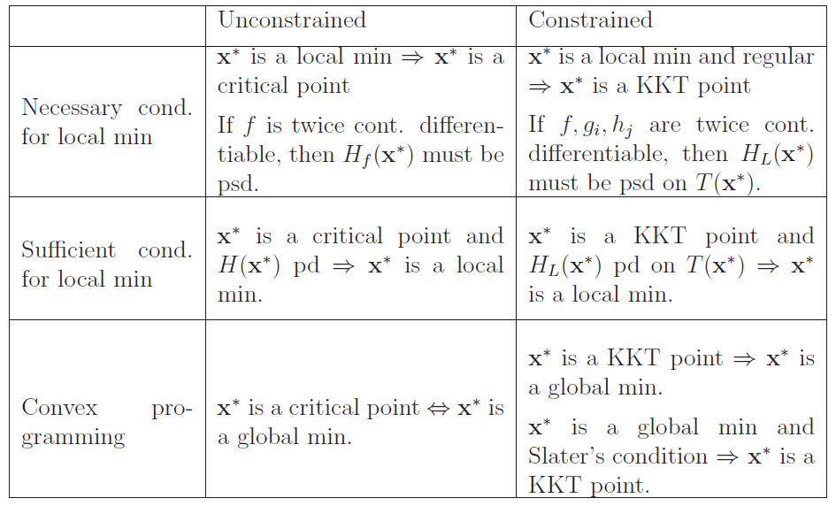
Take form of decomposition-coordination procedure (solution of subproblem is coordinated to solution of global problem)

ADMM : bene fits of dual decomposition + augmented Lagrangian methods for constrained optimization

0 precursor

0.1 Gradient Ascent

Primal problem
$$
\begin{array}{rc}
\min & f(x) \
\text{s.t.} & Ax=b
\end{array}
$$
Lagrangian function is
$$
L(x,y) = f(x) + y^T(Ax-b)
$$
and the dual function is
$$
g(y) = \inf_x L(x,y) = -f^*(-A^Ty) - b^Ty
$$
dual problem is
$$
\max g(y)
$$
recover a primal optimal point $x^*$ from a dual optimal point $y^*$
$$
x^* = \mathop{\mathrm{argmin}}x L(x,y^*)
$$
Solve this dual problem using gradient ascent:
$$
\begin{array}{rl}
x^{k+1} &=& \mathop{\mathrm{argmin}}
{x} L(x,y^k) & x\text{-minimization step} \
y^{k+1} &=& y^k +\alpha^k(Ax^{k+1} - b) & \text{dual variable update}
\end{array}
$$
dual ascent method can lead to a decentralized algorithm in some case.

0.2 Dual Decomposition

If objective $f$ is separable,
$$
f(x) = \sum_{i=1}^N f_i(x_i), \text {where } x=(x_1, \cdots, x_N), \ A = [A_1, \cdots, A_N]
$$
the Lagrangian function is
$$
L(x,y) = \sum_{i=1}^N L_i(x_i,y) = \sum_{i=1}^N (f_i(x_i)+y^TA_ix_i - \frac{1}{N}(y^Tb)
$$
which is separable in $x$. This means that $x$-minimization step splits into $N$ separate problems that can be solved in parallel.

Solve:
$$
\begin{array}{rl}
x_i^{k+1} &=& \mathop{\mathrm{argmin}}_{x_i} L_i(x_i,y^k) & x_i\text{-minimization step} \
y^{k+1} &=& y^k +\alpha^k(Ax^{k+1} - b) & \text{dual variable update}
\end{array}
$$
So, the $x$-minimization step is carried out independently, in parallel.

**Each iteration of the dual decomposition requires a broadcast and gather operation **

[in dual update, collect $A_i x_i^{k+1}$ to compute the residual $Ax^{k+1}-b$. Once global dual variable $y^{k+1}$ is computed, it will be broadcast to $N$ individual $x_i$ minimization steps. ]

  • [Book] Cooperative distributed multi-agent optimization (this book discusses dual decomposition methods and consensus problems).
  • Distributed Dual Averaging in Networks (distributed methods for graph-structured optimization problems)

0.3 Augmented Lagrangians and Method of Multipliers

augmented lagrangian is to bring robustness to dual ascent method, and to yield convergence without assumptions like strict convexity or finiteness of $f$.

Augmented Lagrangian is
$$
L_\sigma(x,y) = f(x) + y^T(Ax-b) + \frac{\sigma}{2} |Ax-b|^2
$$
Dual function is
$$
g_\sigma(y) = \inf_x L_\sigma(x,y)
$$
Adding the penalty term is to be differentiable under rather mild conditions on the original problem.

find gradient of the augmented dual function by minimizing over $x$, then evaluating the resulting equality constraint residual.

Algorithm:
$$
\begin{array}{rl}
x^{k+1} &=& \mathop{\mathrm{argmin}}_{x} L_\sigma(x,y^k) & x\text{-minimization step} \
y^{k+1} &=& y^k +\sigma(Ax^{k+1} - b) & \text{dual variable update}
\end{array}
$$
Here, the parameter $\sigma$ is used as the step size $\alpha^k$.

[The method of multipliers converges under far more general conditions than dual ascent, including cases when $f$ takes on the value $+\infty$ or is not strictly convex.]

  • How to choose $\sigma$:

    The optimality condition are primal and dual feasibility, i.e.,
    $$
    Ax^* - b = 0, \quad \nabla f(x^*) + A^Ty^* = 0
    $$
    Then, we have $x^{k+1}$ can minimize $L_\sigma(x,y^k)$, so
    $$
    \begin{aligned}
    0 &= \nabla_x L_\sigma(x^{k+1}, y^k) \
    &= \nabla_x f(x^{k+1}) + A^T(y^k + \sigma(Ax^{k+1}-b)) \
    &= \nabla_x f(x^{k+1}) + A^T y^{k+1}
    \end{aligned}
    $$
    So, using $\sigma$ as step size in dual update, the iterate $(x^{k+1}, y^{k+1})$ is dual feasible. $\rightarrow$ primal residual $Ax^{k+1}-b$ converges to 0. $\rightarrow$ optimality.

Shortcoming: When $f$ is separable, the augmented Lagrangian $L_\sigma$ is not separable, so the $x$-minimization step cannot be carried out separately in parallel for each $x_i$. This means that the basic method of multipliers cannot be used for decomposition

1. ADMM

blend the decomposability of dual ascent with the superior convergence properties of the method of multipliers.

Problem:
$$
\begin{array}{rcl}
\min & f(x)+g(z) \
\text{s.t. } & Ax+Bz = c
\end{array}
$$
difference: $x$ splits into two parts, $x$ and $z$, with the objective function separable across the splitting.

optimal value:
$$
p^* = \inf { f(x)+g(z) | Ax+Bz = c }
$$
Augmented Lagrangian:
$$
L_\sigma (x,z;y) = f(x)+g(z)+y^T(Ax+Bz-c)+\frac{\sigma}{2} |Ax+Bz-c|^2
$$

1.1 Algorithm

1.1.1 Unscaled form

$$
\begin{aligned}
x^{k+1} &= \mathop{\mathrm{argmin}}_x L_\sigma(x,z^k,y^k) & x\text{-minimization}\
z^{k+1} &= \mathop{\mathrm{armmin}}_z L_\sigma(x^{k+1},z,y^k) & z\text{-minimization}\
y^{k+1} &= y^k + \sigma(Ax^{k+1}+Bz^{k+1}-c) & \text{dual variable update}
\end{aligned}
$$

why ADMM is alternating direction:

If use method of multipliers to solve this problem, we will have
$$
\begin{aligned}
(x^{k+1}, z^{k+1}) &= \mathop{\mathrm{argmin}}_{x,z} L_\sigma(x,z,y^k) \
y^{k+1} &= y^k + \sigma(Ax^{k+1}+Bz^{k+1}-c)
\end{aligned}
$$
So, the augmented lagrangian is minimized jointly with two variables $x,z$.

But, ADMM update $x$ and $z$ in an alternating or sequential fashion, –> alternating direction.

ADMM can be viewed as a version of method of multipliers where a single Gauss-Seidel pass over $x$ and $z$ is used instead of joint minimization.

1.1.2 Scaled form

combine the linear and quadratic terms in the augmented lagrangian and scale the residual variable.

Set $u = \frac{1}{\sigma} y$, the ADMM becomes
$$
\begin{array}{l}
{x^{k+1}:=\underset{x}{\operatorname{argmin}} \left(f(x) + \frac{\sigma}{2} \left|A x+B z^{k}-c+u^{k}\right|^{2}\right)} \
{z^{k+1}:=\underset{z}{\operatorname{argmin}} \left(g(z) + \frac{\sigma}{2} \left|A x^{k+1}+B z-c+u^{k}\right|^{2}\right)} \
{u^{k+1}:=u^{k}+A x^{k+1}+B z^{k+1}-c}\end{array}
$$
Define residual at $k$ iteration as $r^k=Ax^k+Bz^k-c$, we have
$$
u^k = u^0 + \sum_{j=1}^k r^j
$$

1.2 Convergence

Assumption 1:

function $f: \mathbb R^n \rightarrow \mathbb R \cup {+\infty}$ and $g: \mathbb R^m \rightarrow \mathbb R \cup {+\infty}$ are closed, proper and convex

this assumption means the subproblem in $x$-update and $z$-update are solvable.

allows $f$ and $g$ are nondifferentiable and to assume value $+\infty$. For example, $f$ is indicator function

Assumption 2:

Unaugmented Lagrangian $L_0$ has a saddle point. This means there exists $(x^*, z^*, y^*)$ such that
$$
L_0 (x^*, z^*, y) \leq L_0(x^*, z^*, y^*) \leq L_0(x^*, z^*, y^*)
$$

Based on assumption1, $L_0(x^*, z^*, y^*)$ is finite for saddle point $(x^*, z^*, y^*)$. So, $(x^*, z^*)$ is solution to $\mathrm{argmin}_{x,z} L(x,z,y)$. So, $Ax^* + Bz^* = c$ and $f(x^*)<\infty$, $g(z^*)<\infty$. =

It also implies that $y^*$ is dual optimal, and the optimal value of the primal and dual problem are equal, i.e., the strong duality holds.

Under Assumption 1 and Assumption 2, ADMM iteration satisfy:

  • residual convergence: $r^k \rightarrow 0$ as $k\rightarrow \infty$.
  • objective convergence: $f(x^k)+g(z^k) \rightarrow p^*$ as $k\rightarrow \infty$.
  • dual variable convergence: $y^k \rightarrow y^*$ as $k\rightarrow \infty$.

1.3 Optimality condition and Stopping creterion

1.3.1 Optimality condition for ADMM:

  1. Primal feasibility
    $$
    Ax^* + Bz^* -c = 0
    $$
  2. Dual feasibility
    $$
    \begin{aligned}
    0 &\in \part f(x^*) + A^Ty^* \
    0 &\in \part g(z^*) + B^Ty^*
    \end{aligned}
    $$

Since $z^{k+1}$ minimizes $L_\sigma(x^{k+1},z,y^k)$, we have
$$
0\in \part g(z^{k+1}) + B^T y^k + \sigma B^T(Ax^{k+1}+Bz^{k+1}-c)\
= \part g(z^{k+1}) + B^T y^k + \sigma B^T r^{k+1} \
= \part g(z^{k+1}) + B^T y^k
$$
This means that $z^{k+1}$ and $y^{k+1}$ satisfy $0\in \part g(z^*)+ B^T u^*$. Similarly, can obtain other conditions.

the last condition holds for $(x^{k+1}, z^{k+1}, y^{k+1})$, the residual for the other two are primal and dual residuals $r^{k+1}$ and $s^{k+1}$.

1.3.2 Stopping criteria

suboptimality
$$
f(x^k)+g(z^k)-p^* \leq -(y^k)^Tr^k + (x^k-x^*)^T s^k
$$
shows that when the residuals $r^k$ and $s^k$ are small, the objective suboptimality will be small.

It’s hard to use this inequality as stopping criterion. But if we guess $|x^k-x^* | \leq d$, we have
$$
f(x^k)+g(z^k)-p^* \leq -(y^k)^Tr^k + d |s^k| \leq |y^k| |r^k| + d|s^k|
$$
so, the stopping criterion is that the primal and dual residual are small, i.e.,
$$
|r^k| \leq \epsilon^{\mathrm {pri}} \quad \text{and } \quad |s^k| \leq \epsilon^{\text{dual}}
$$
where $\epsilon^{\text{pri}}, \epsilon^{\text{dual}}$ are feasibility tolerance for primal and dual feasibility conditions. These tolerance can be chosen using an absolute and relative criterion, such as
$$
\begin{aligned}
\epsilon^{\text{pri}} &= \sqrt{p} \epsilon^{\text{abs}} + \epsilon^{\text{rel}} \max{ |Ax^k|, B|z^k|, |c| }, \
\epsilon^{\text{dual}} &= \sqrt{n} \epsilon^{\text{abs}} + \epsilon^{rel} |A^Ty^k|
\end{aligned}
$$

1.4 Extension and Variations

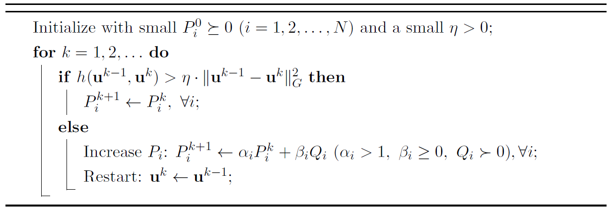
  1. Varying Penalty Parameter

    using different penalty parameters $\sigma^k$ for each iteration. -> improve convergence, reduce independence on initial $\sigma$.
    $$
    \sigma^{k+1}:=\left{\begin{array}{ll}
    {\tau^{\text {incr }} \sigma^{k}} & {\text{if } |r^{k}| > \mu |s^{k}|} \
    {\sigma^{k} / \tau^{\text {decr }}} & {\text {if }|s^{k}| > \mu |r^{k}|} \
    {\sigma^{k}} & {\text { otherwise }}
    \end{array}\right.
    $$
    where $\mu>1, \tau^{\text{incr}}>1, \tau^{\text{decr}}>1$ are parameters.

    The idea behind this penalty parameter update is to try to keep the primal and dual residual norms within a factor of $\mu$ of one another as they both converge to zero.

    • large values of $\sigma$ place a large penalty on violations of primal feasibility and so tend to produce small primal residuals.

    • Conversely, small values of $\sigma$ tend to reduce the dual residual, but at the expense of reducing the penalty on primal feasibility, which may result in a larger primal residual.

    So, when primal residual becomes large, inflates $\sigma$ by $\tau^{\text{incr}}$; when primal residual seems too small, deflates $\sigma$ by $\tau^{\text{decr}}$.

    When a varying penalty parameter is used in the scaled form of ADMM, the scaled dual variable $u^k=\frac{1}{\sigma} y^k$ should be rescaled after updating $\sigma$.

  2. More general Augmenting terms

    • idea 1: use different penalty parameters for each constraint,
    • idea 2: replace the quadratic term $\frac{\sigma}{2} |r|^2$ with $\frac{1}{2} r^TPr$, where $P$ is a symmetric positive definite matrix.
  3. Over-relaxation in the $z$- and $y$- updates, $Ax^{k+1}$ can be replaced with
    $$
    \alpha^k Ax^{k+1} - (1-\alpha^k) (Bz^k-c)
    $$

    where $\alpha^k \in (0,2)$ is a relaxation parameter. When $\alpha^k >1$, over-relaxation; when $\alpha^k<1$, under-relaxation.

  4. Inexact minimization

    ADMM will converge even when the $x$- and $z$-minimization steps are not carried out exactly, provided certain suboptimality measures in the minimizations satisfy an appropriate condition, such as being summable.

    in situations where the x- or z-updates are carried out using an iterative method; it allows us to solve the minimizations only approximately at first, and then more accurately as the iterations progress

  5. Update ordering

    $x$-, $y$-, $z$- updates in varying orders or multiple times.

    for example:

    divide variables into $k$ blocks and update each of them in turn (multiple times). –> multiple Gauss-Seidel passes.

  6. Related algorithms

    Dual ADMM [80]: applied ADMM to a dual problem.

    Distributed ADMM [183]:

    combination ADMM and proximal method of multipliers.

2. General Patterns

Three cases:

  • quadratic objective terms;
  • separable objective and constraints;
  • smooth objective terms.

Here, we just discuss $x$-update, and can be easily applied to $z$-update.
$$
x^+ = \mathop{\mathrm{argmin}}_x (f(x)+\frac{\sigma}{2} |Ax-v|^2)
$$
where $v=-Bz+c-u$ is a known constant vector for the purpose of the $x$-update.

2.1 Proximity Operator

If $A=I$, $x$-update is
$$
x^+ = \mathop{\mathrm{argmin}}x (f(x)+\frac{\sigma}{2} |x-v|^2) = \mathrm{Prox}{f,\sigma}(v)
$$
Moreau envelope or MY regularization of $f$:
$$
\tilde f(v) = \inf_x (f(x)+\frac{\sigma}{2} |x-v|^2 )
$$
So, the $x$-minimization in the proximity operator is called proximal minimization.

for example: if $f$ is the indicator function of set $\mathcal C$, the $x$-update is
$$
x^+ = \mathop{\mathrm{argmin}}x (f(x)+\frac{\sigma}{2} |x-v|^2) = \Pi{\mathcal C}(v)
$$

2.2 Quadratic Objective Terms

$$
f(x) = \frac{1}{2} x^TPx+q^Tx+r
$$

where $P\in \mathbb S^n_+$, the set of symmetric positive semidefinite $n\times n$ matrices.

Assume $P+\sigma A^TA$ is invertible, $x^+$ is an affine function of $v$ given by
$$
x^+ = (P+\sigma A^TA)^{-1} (\sigma A^Tv-q)
$$

  1. direct methods:

If we want to solve $Fx=g$, steps:

  1. factoring $F = F_1F_2\cdots F_k$

  2. back-solve: solve $F_iz_i=z_{i-1}$ where $z_1=F_1^{-1}g$ and $x=z_k$

    (given $z_1$, can compute $z_2$ based on $F_2z_2 =z_1$, then iterates, so can compute $z_k$, i.e., can compute $x$).

The cost of solving $Fx = g$ is the sum of the cost of factoring $F$ and the cost of the back-solve.

​ In our case, $F=P+\sigma A^TA, \ g=\sigma A^Tv-q$, where $P\in \mathbb S_+^n, A\in \mathbb R^{p\times n}$.

We can form $F = P + \sigma A^TA$ at a cost of $O(pn^2)$ flops (floating point operations). We then carry out a Cholesky factorization of $F$ at a cost of $O(n^3)$ flops; the back-solve cost is $O(n^2)$. (The cost of forming $g$ is negligible compared to the costs listed above.) When $p$ is on the order of, or more than $n$, the overall cost is $O(pn^2)$. (When $p$ is less than $n$ in order, the matrix inversion lemma described below can be used to carry out the update in $O(p^2n)$ flops.)

  1. Exploiting Sparsity

    When $A$ and $P$ can make $F$ sparse. can be more efficient

  2. Caching Factorizations

    $Fx^{(i)}=g^{(i)}$, If $t$ is the factorization cost and $s$ is the back-solve cost, then the total cost becomes $t + Ns$ instead of $N(t + s)$, which would be the cost if we were to factor $F$ each iteration. As long as $\sigma$ does not change, we can factor $P + \sigma A^TA$ once, and then use this cached factorization in subsequent solve steps

  3. Matrix Inversion Lemma
    $$
    \left(P+\sigma A^{T} A\right)^{-1}=P^{-1}-\sigma P^{-1} A^{T}\left(I+\sigma A P^{-1} A^{T}\right)^{-1} A P^{-1}
    $$
    For efficient computation.

  4. Quadratic Function restricted to an Affine Set
    $$
    f(x)=(1 / 2) x^{T} P x+q^{T} x+r, \quad \text { dom } f={x | F x=g}
    $$
    Here, $x^+$ is still an affine function of $v$. the update involves solving the KKT condition:
    $$
    \left[\begin{array}{cc}{P+\sigma I} & {F^{T}} \ {F} & {0}\end{array}\right]\left[\begin{array}{c}{x^{k+1}} \ {\nu}\end{array}\right]+\left[\begin{array}{c}{q-\sigma\left(z^{k}-u^{k}\right)} \ {-g}\end{array}\right]=0
    $$
    ==So, here, A=I​?==

2.3 Smooth Objective Terms

If $f$ is smooth, can use iterative methods. (gradient method, nonlinear conjugate gradient, L-BFGS)

The convergence of these methods depends on the conditioning of the function to be minimized. The presence of the quadratic penalty term $\frac{\sigma}{2} |Ax-v|^2$ tends to improve the conditioning of the problem and thus improve the performance of an iterative method for updating $x$.

Can adjust $\sigma$ in each iteration to converges quichly.

  1. Early Termination

    Early termination in the $x$- or $z$-updates can result in more ADMM iterations, but much lower cost per iteration, giving an overall improvement in efficiency.

  2. Warm Start

    initialize the iterative method used in the $x$-update at the solution $x^k$ obtained in the previous iteration

  3. Quadratic Objective Terms

    worth using an iterative method than a direct method. –> conjugate gradient method.

    Can use when direct method do not work, or $A$ is dense.

2.4 Decomposition

  1. Block Separability

    $x=(x_1, \cdots, x_N)$, then $f(x)=f_1(x_1) + \cdots +f_N(x_N)$. If the quadratic term $|Ax|^2$ is also separable, i.e., $A^TA$ is block diagonal, then the augmented lagrangian $L_\sigma$ is separable. –> compute in parallel.

  2. Component separability

    $f(x)=f_1(x_1) + \cdots +f_n(x_n)$ and $A^TA$ is diagonal. $x$-minimization step can be carried out via $n$ scalar minimization.

  3. Soft Thresholding

    If $f(x)=\lambda ||x|1$ and $A=I$, –> component separability. the scalar $x_i$-update is
    $$
    x_i^+ = \mathop{\operatorname{argmin}}
    {x_i}(\lambda |x_i| + \frac{\sigma}{2}(x_i-v_i)^2)
    $$
    Even the first term is not differentiable, But can use subdifferential.
    $$
    \begin{array}{ll}
    &x_i^+ = S_{\frac{\lambda}{\sigma}} (v_i)& \
    \text{where }& & \
    &S_\kappa(a) = \begin{cases} a-\kappa,\quad& a>\kappa \ 0, \quad& |a|\leq \kappa \
    a+\kappa, \quad& a< -\kappa\end{cases} \text{ or } S_\kappa(a) = (a-\kappa)- - (-a-\kappa)+
    \end{array}
    $$
    Actually, this is proximity operator of the $\ell_1$ norm.

3. Constrained Convex Optimization

3.1.1 Alternating Projection

find intersection of two sets.

alternating projection:
$$
\begin{array}{l}{x^{k+1}:=\Pi_{\mathcal{C}}\left(z^{k}\right)} \ {z^{k+1}:=\Pi_{\mathcal{D}}\left(x^{k+1}\right)}\end{array}
$$
ADMM:
$$
\begin{array}{ll}
\min & f(x)+g(z) \
\text{s.t. } & x-z = 0
\end{array}
$$
where $f$ and $g$ are indicator function of $\mathcal C$ and $\mathcal D$.
$$
\begin{array}{l}{x^{k+1}:=\Pi_{\mathcal{C}}\left(z^{k}-u^k\right)} \ {z^{k+1}:=\Pi_{\mathcal{D}}\left(x^{k+1}+u^k\right)} \
u^{k+1} := u^k+x^{k+1}-z^{k+1} \end{array}
$$
This ADMM method is more efficient than previous method.

3.1.2 Parallel Projection

find a point in the intersection of $N$ sets $\mathcal A_1, \cdots, \mathcal A_N$.

So, $\mathcal C=\mathcal A_1\times \cdots \times \mathcal A_N$, $\mathcal D={(x_1, \cdots, x_N) \in \mathbb R^{nN} | x_1 = \cdots = x_N }$.

So, $\Pi_\mathcal C(x) = (\Pi_{\mathcal A_1}(x_1), \cdots, \Pi_{\mathcal A_N}(x_N))$, $\Pi_\mathcal D(x)=(\bar x, \cdots, \bar x)$, where $\bar x = \frac{1}{N}\sum_{i=1}^N x_i$.

each step of ADMM can be carried out by projecting points onto each of the sets $\mathcal A_i$ in parallel and then averaging the results:
$$
\begin{aligned} x_{i}^{k+1} &:=\prod_{\mathcal{A}{i}}\left(z^{k}-u{i}^{k}\right) \ z^{k+1} &:=\frac{1}{N} \sum_{i=1}^{N}\left(x_{i}^{k+1}+u_{i}^{k}\right) \ u_{i}^{k+1} &:=u_{i}^{k}+x_{i}^{k+1}-z^{k+1} \end{aligned}
$$
The first and third steps can be carried out in parallel.

indicator function of $\mathcal A_1 \cap \cdots \cap \mathcal A_N$ splits into the sum of the indicator functions of each $\mathcal A_i$.

Another compact representation:
$$
\begin{array}{ll}
&x_i^{k+1} = \Pi_{\mathcal A_i}(\bar x^k - u_i^k) \
&u_i^{k+1} = u_i^k + (x_i^{k+1}-\bar x^{k+1}) \
\text{where} & \bar u^{k+1}=\bar u^k+\bar x^{k+1}- z^k, z^{k+1} = \bar x^{k+1}+\bar u^k
\end{array}
$$
This shows that the $u_i^k$ is the running sum of the discrepancies $x_i^k-\bar x^k$. The first step is a parallel projection onto the sets $\mathcal C_i$; the second involves averaging the projected points.

3.2 Linear and Quadratic Programming

Quadratic program (QP)
$$
\begin{array}{rc}
\min & \frac{1}{2}x^TPx + q^Tx \
\text{s.t. } & Ax=b, x\ge 0
\end{array}
$$
where $x\in \mathbb R^n$, $P\in \mathbb S_+^n$.

Represent it as ADMM form as
$$
\begin{array}{rcc}
&\min & f(x)+g(z) \
&\text{s.t. } & x-z=0 \
\text{where, } & &f(x)=\frac{1}{2}x^TPx + q^Tx, & \mathrm{dom} f={x|Ax=b}, & g(z)=\delta_{\mathbb R_+^n}(z)
\end{array}
$$
$f$ is the original objective with restricted domain and $g$ is the indicator function of $\mathbb R_+^n$.

Scaled form of ADMM:
$$
\begin{aligned}
x^{k+1} &:=\operatorname{argmin}{x}\left(f(x)+\frac{\sigma}{2} \left|x-z^{k}+u^{k}\right|^{2}\right) \
z^{k+1} &:=\left(x^{k+1}+u^{k}\right)
{+} \
u^{k+1} &:=u^{k}+x^{k+1}-z^{k+1}
\end{aligned}
$$
Here, the $x$-update is an equality-constrained least square problem with optimality KKT conditions, $\nu$ is multiplier.
$$
\begin{bmatrix}{P+\sigma I} & {A^{T}} \ {A} & {0}\end{bmatrix} \begin{bmatrix}{x^{k+1}} \ {\nu}\end{bmatrix} + \begin{bmatrix}{q-\sigma\left(z^{k}-u^{k}\right)} \ {-b}\end{bmatrix} = 0
$$

Linear and Quadratic Cone Programming

conic constraint $x\in \mathcal K$ to replace $x\ge 0$ above

The only change to ADMM is the $z$-update (Projection onto $\mathcal K$)

For example, we can solve a semidefinite program with $x \in \mathbb S^n_+$ by projecting $x^{k+1} + u^k$ onto $\mathbb S^n_+$ using an ==eigenvalue decomposition==.

4. $\ell_1$ Norm Problems

ADMM explicitly targets problems that split into two distinct parts, $f$ and $g$, that can then be handled separately.

ADMM can decouple the nonsmooth $\ell_1$ term from the smooth loss term.

4.1 Least Absolute Deviations

minimize $|Ax-b|_1$ instead of $|Ax-b|_2^2$. provide a more robust fit than least squares

ADMM form:
$$
\begin{array}{ll}
\min & |z|_1 \
\text{s.t. } & Ax-z=b
\end{array}
$$
so, $f=0$, $g=| \cdot|_1$.

ADMM algorithm:
$$
\begin{aligned}
x^{k+1} &:= (A^TA)^{-1} A^T (b+z^k-u^k) \
z^{k+1} &:= S_{\frac{1}{\sigma}}(Ax^{k+1}-b+u^k) \
u^{k+1} &:= u^{k} + Ax^{k+1} - z^{k+1} - b
\end{aligned}
$$

  1. Huber fitting

    between least square and lease absolute.
    $$
    \begin{array}
    {} &\min & g^{\text{hub}}(Ax-b) \
    \text{where} & &g^{\text{hub}}(a)= \begin{cases} \frac{a^2}{2},\quad & |a|\le 1 \ |a|-\frac{1}{2},\quad & |a|>1 \end{cases} &
    \end{array}
    $$

    ADMM algorithm:

    same. Only difference is the $z$-update
    $$
    z^{k+1}:=\frac{\sigma}{1+\sigma}\left(A x^{k+1}-b+u^{k}\right)+\frac{1}{1+\sigma} S_{1+1 / \sigma}\left(A x^{k+1}-b+u^{k}\right)
    $$

4.2 Basis Pursuit

$$
\begin{array}{ll}
\min & |x|_1 \
\text{s.t. } & Ax=b
\end{array}
$$

with $x\in \mathbb R^n$, $A\in \mathbb R^{m\times n}$, $b\in \mathbb R^m$ ($m<n$).

Aim: to find a sparse solution to an underdetermined system with equality equations.

ADMM form:
$$
\begin{array}{ll}
\min & f(x)+|z|_1 \
\text{s.t. } & x-z=0
\end{array}
$$
where $f$ is indicator function of set $\mathcal C={x\in \mathbb R^n | Ax=b}$.

ADMM algorithm:
$$
\begin{aligned}
x^{k+1} &:= \Pi_\mathcal C (z^k-u^k) \
z^{k+1} &:= S_{\frac{1}{\sigma}}(x^{k+1}+u^k) \
u^{k+1} &:= u^{k} + x^{k+1} - z^{k+1}
\end{aligned}
$$
The subproblem of $x$-update is solving a linearly-constrained minimum Euclidean norm problem


$$
x^{k+1} = (I-A^T (AA^T)^{-1} A)(z^k-u^k) + A^T(AA^T)^{-1}b
$$

4.3 General $\ell_1$ regularized loss minimization

Problem: $\min \quad l(x)+\lambda |x|_1$

ADMM form:
$$
\begin{array}{rll}
&\min & l(x)+g(z) \
&\text{s.t. } & x-z=0 \
\text{where,} & & g(z)=\lambda |z|1
\end{array}
$$
ADMM algorithm:
$$
\begin{aligned}
x^{k+1} &:=\operatorname{argmin}
{x}\left(l(x)+\frac{\sigma}{2} \left|x-z^{k}+u^{k}\right|^{2}\right) \
z^{k+1} &:= S_{\frac{\lambda}{\sigma}}(x^{k+1}+u^k) \
u^{k+1} &:=u^{k}+x^{k+1}-z^{k+1}
\end{aligned}
$$
For subproblem $x$-update:

  • If $l$ is smooth, this can be done by any standard method, such as Newton’s method, a quasi-Newton method such as L-BFGS, or the conjugate gradient method.
  • If $l$ is quadratic, the $x$-minimization can be carried out by solving linear equations

4.2 Lasso

$$
\min \frac{1}{2} |Ax-b|^2 + \lambda |x|_1
$$

ADMM form:
$$
\begin{array}{rll}
&\min & f(x)+g(z) \
&\text{s.t. } & x-z=0 \
\text{where,} & & f(x)=\frac{1}{2}|Ax-b|^2,\quad g(z)=\lambda |z|1
\end{array}
$$
ADMM algorithm:
$$
\begin{aligned}
x^{k+1} &:= (A^TA+\sigma I)^{-1} (A^Tb+\sigma(z^k-u^k)) \
z^{k+1} &:= S
{\frac{\lambda}{\sigma}}(Ax^{k+1}-b+u^k) \
u^{k+1} &:= u^{k} + Ax^{k+1} - z^{k+1}
\end{aligned}
$$

4.4.1 Generalized Lass

$$
\min \frac{1}{2} |Ax-b|^2 + \lambda |Fx|_1
$$

where $F$ is an arbitrary linear transformation.

==Special cases:==
$$
F_{ij}=\begin{cases} 1, \quad & j=i+1 \ -1, \quad & j=i \ 0, \quad & \text{otherwise} \end{cases}
$$
and $A=I$, the generation reduces to
$$
\min \frac{1}{2} |x-b|^2 + \lambda \sum_{i=1}^{n-1} |x_{i+1}-x_i|
$$

ADMM form:
$$
\begin{array}{rll}
&\min & \frac{1}{2} |Ax-b|^2 + \lambda |z|1\
&\text{s.t. } & Fx-z=0 \
\end{array}
$$
ADMM algorithm:
$$
\begin{aligned}
x^{k+1} &:= (A^TA+\sigma F^TF)^{-1} (A^Tb+\sigma F^T(z^k-u^k)) \
z^{k+1} &:= S
{\frac{\lambda}{\sigma}}(Fx^{k+1}+u^k) \
u^{k+1} &:= u^{k} + Fx^{k+1} - z^{k+1}
\end{aligned}
$$

For the previous special case, the $A^TA+\sigma F^TF$ is tridiagonal, so can be carried out in $O(n)$ flops.

4.4.2 Group Lasso

Replace $|x|1$ with $\sum{i=1}^N |x_i|_2$ where $x=(x_1, \cdots, x_N)$ with $x_i \in \mathbb R^{n_i}$.

All the same, except the $z$-update:
$$
z_i^{k+1} := S_{\frac{\lambda}{\sigma}}(x_i^{k+1}+u^k), \quad o=1, \cdots, N \
$$
where the thresholding operator $S_\kappa$ is
$$
S_\kappa(a)=(1-\frac{\kappa}{|a|2} )+ a
$$

Extend to handle the overlapping groups.

$N$ potentially overlapping groups $G_i \subseteq {1,\cdots, n}$, the objective is
$$
\frac{1}{2} |Ax-b|^2 + \lambda \sum_{i=1}^N |x_{G_i} |
$$
because the groups can overlap, this kind of objective is difficult to optimize with many standard methods, but it is straightforward with ADMM.

ADMM: Introduce $x_i\in \mathbb R^{|G_i|}$ and consider problem:
$$
\begin{array}{ll}
\min & \frac{1}{2} |Az-b|^2 + \lambda \sum_{i=1}^N |x_i| \
\text{s.t. } & x_i-\tilde z_i=0, i=1, \cdots, N
\end{array}
$$

Sparse Inverse Covariance Selection

5. Consensus and Sharing

$$
\min f(x) = \sum_{i=1}^N f_i(x)
$$

5.1 Global Variable Consensus

Global consensus problem:

add global consensus variable $z$ to split the minimization problem
$$
\begin{aligned}
\min \quad& \sum_{i=1}^N f_i(x_i) \
\text{s.t.} \quad& x_i-z = 0, \ i=1,\cdots,N
\end{aligned}
$$

constraint means all the local variables $x_i$ should be equal.

Augmented Lagrangian:
$$
L_\sigma(x_1, \cdots, x_N, z, y) = \sum_{i=1}^N \left( f_i(x_i) + y_i^T(x_i-z) + \frac{\sigma}{2} |x_i-z|^2 \right)
$$
constraint set is
$$
\mathcal C = {(x_1, \cdots, x_N) | x_1=x_2=\cdots=x_N }
$$
ADMM algorithm:
$$
\begin{aligned}
x_i^{k+1} &:= \mathop{\mathrm{argmin}}{x_i} \left( f_i(x_i)+y_i^{kT}(x_i-z^k)+\frac{\sigma}{2}|x_i-z^k|^2 \right) \
z^{k+1} &:= \frac{1}{N} \sum
{i=1}^N \left( x_i^{k+1} + \frac{1}{\sigma}y_i^k \right) \
y_i^{k+1} &:= y^k_i + \sigma(x_i^{k+1}-z^{k+1})
\end{aligned}
$$
Here, the first and last step can be carried out independently.

Simplify this algorithm:
$$
\begin{array}{ll}
&\begin{aligned}
x_i^{k+1} &:= \mathop{\mathrm{argmin}}_{x_i} \left( f_i(x_i)+y_i^{kT}(x_i-z^k)+\frac{\sigma}{2}|x_i-\bar x^k|^2 \right) \
y_i^{k+1} &:= y^k_i + \sigma(x_i^{k+1}-\bar x^{k+1})
\end{aligned} \
\text{where, } & \quad z^{k+1} = \bar x^{k+1} + \frac{1}{\sigma} \bar y^k \
\end{array}
$$
The dual variables are separately updated to drive the variables into consensus, and quadratic regularization helps pull the variables toward their average value while still attempting to minimize each local $f_i$.

We can interpret consensus ADMM as a method for solving problems in which the objective and constraints are distributed across multiple processors. Each processor only has to handle its own objective and constraint term, plus a quadratic term which is updated each iteration. The quadratic terms (or more accurately, the linear parts of the quadratic terms) are updated in such a way that the variables converge to a common value, which is the solution of the full problem.

Primal and dual residual are
$$
{r^{k}=\left(x_{1}^{k}-\bar{x}^{k}, \ldots, x_{N}^{k}-\bar{x}^{k}\right), \quad s^{k}=-\sigma\left(\bar{x}^{k}-\bar{x}^{k-1}, \ldots, \bar{x}^{k}-\bar{x}^{k-1}\right)}
$$
So, the square norms are
$$
{\qquad\left|r^{k}\right|{2}^{2}=\sum{i=1}^{N}\left|x_{i}^{k}-\bar{x}^{k}\right|{2}^{2}, \quad\left|s^{k}\right|{2}^{2}=N \sigma^{2}\left|\bar{x}^{k}-\bar{x}^{k-1}\right|_{2}^{2}}
$$

5.1.2 Global Variable Consensus with Regularization

$$
\begin{array}{ll}
\min & \sum_{i=1}^N f_i(x_i) + g(z) \
\text{s.t. } & x_i-z=0, i=1,\cdots, N
\end{array}
$$

ADMM algorithm:
$$
\begin{array}{l}{x_{i}^{k+1}:=\underset{x_{i}}{\operatorname{argmin}}\left(f_{i}\left(x_{i}\right)+y_{i}^{k T}\left(x_{i}-z^{k}\right)+\frac{\sigma}{2} \left|x_{i}-z^{k}\right|{2}^{2}\right)} \ {z^{k+1}:=\underset{z}{\operatorname{argmin}}\left(g(z)+\sum{i=1}^{N}\left(-y_{i}^{k T} z+\frac{\sigma}{2} \left|x_{i}^{k+1}-z\right|{2}^{2}\right)\right)} \ {y{i}^{k+1}:=y_{i}^{k}+\sigma\left(x_{i}^{k+1}-z^{k+1}\right)} \end{array}
$$
Express the $z$-update as an averaging step, so we can have
$$
{\quad z^{k+1}:=\underset{z}{\operatorname{argmin}}\left(g(z)+\frac{N\sigma}{2}\left|z-\bar{x}^{k+1}-\frac{1}{\sigma} \bar{y}^{k}\right|_{2}^{2}\right)}
$$

example 1:

$g(z)=\lambda |z|1$, $z$-update becomes $z^{k+1}:=S{\frac{\lambda}{N\sigma}}(\bar x^{k+1}-\frac{1}{\sigma} \bar y^k)$

Example 2:

$g$ is indicator function of $\mathbb R^n_+$, i.e., $g=\delta_{\mathbb R_+^n}$. $z$-update is $z^{k+1}:=(\bar x^{k+1}-\frac{1}{\sigma} \bar y^k)_+$

Algorithm:
$$
\begin{array}{l}{x_{i}^{k+1}:=\underset{x_{i}}{\operatorname{argmin}}\left(f_{i}\left(x_{i}\right)+\frac{\sigma}{2} \left|x_{i}-z^{k}+u_i^k\right|{2}^{2}\right)} \
{z^{k+1}:=\underset{z}{\operatorname{argmin}}\left(g(z)+\frac{N\sigma}{2} \left|z-x
{i}^{k+1}-\bar u^k\right|{2}^{2}\right)} \
{u
{i}^{k+1}:=u_{i}^{k}+x_{i}^{k+1}-z^{k+1}} \end{array}
$$

5.2 General Form Consensus Optimization

Objective: $f_1(x_1) + \cdots + f_N(x_N)$. Each of these local variables consists of a selection of the components of the global variables $z\in \mathbb R^n$. This means each components of local variable corresponds to some global variable component $z_g$.

Mapping from local to global: $g=\mathcal G(i,j)$

In the context of model fitting, the following is one way that general form consensus naturally arises. The global variable $z$ is the full feature vector (i.e., vector of model parameters or independent variables in the data), and different subsets of the data are spread out among $N$ processors. Then xi can be viewed as the subvector of $z$ corresponding to (nonzero) features that appear in the $i$th block of data. In other words, each processor handles only its block of data and only the subset of model coefficients that are relevant for that block of data. If in each block of data all regressors appear with nonzero values, then this reduces to global consensus.

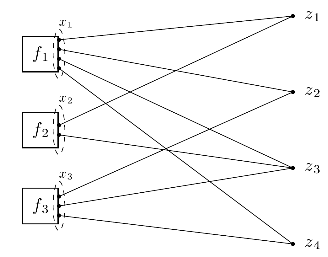
$\tilde z_i \in \mathbb R^{n_i}$ defined by $(\tilde z_i)j = z{\mathcal G(i,j)}$.

General form consensus problem is
$$
\begin{array}{ll}
\min & \sum_{i=1}^N f_i(x_i) \
\text{s.t. }& x_i-\tilde z_i = 0, i = 1, \cdots, N
\end{array}
$$
Augmented Lagrangian is
$$
L_\sigma(x,z,y) = \sum_{i=1}^N \left( f_i(x_i) + y^T_i(x_i-\tilde z_i) + \frac{
\sigma}{2} |x_i - \tilde z_i |^2 \right)
$$
with the dual variables $y_i\in \mathbb R^{n_i}$.

ADMM algorithm:
$$
\begin{array}{l}
{x_{i}^{k+1}:=\underset{x_{i}}{\operatorname{argmin}}\left(f_{i}\left(x_{i}\right)+y_{i}^{k T}x_{i}+\frac{\sigma}{2} \left|x_{i}-\tilde z_i^{k}\right|{2}^{2}\right)} \ {z^{k+1}:=\underset{z}{\operatorname{argmin}}\left(\sum{i=1}^{m}\left(-y_{i}^{k T} \tilde z_i+\frac{\sigma}{2} \left|x_{i}^{k+1}-\tilde z_i\right|{2}^{2}\right)\right)} \ {y{i}^{k+1}:=y_{i}^{k}+\sigma\left(x_{i}^{k+1}-\tilde z_i^{k+1}\right)}
\end{array}
$$
where $x_i$- and $y_i$- updates can be carried out independently for each $i$.

The $z$- update step decouples across the components of $z$, since $L_\sigma$ is fully separable in its components:
$$
z_{g}^{k+1}:=\frac{\sum_{\mathcal{G}(i, j)=g}\left(\left(x_{i}^{k+1}\right){j}+(1 / \sigma)\left(y{i}^{k}\right){j}\right)}{\sum{\mathcal{G}(i, j)=g} 1}
$$

the $z$-update is local averaging for each component $z_g$ rather than global averaging;

in the language of collaborative filtering, we could say that only the processing elements that have an opinion on a feature $z_g$ will vote on $z_g$.

5.2.1 General Form Consensus with Regularization

$$
\begin{array}{ll}
\min & \sum_{i=1}^N f_i(x_i) + g(z) \
\text{s.t. }& x_i-\tilde z_i = 0, i = 1, \cdots, N
\end{array}
$$

where $g$ is a regularization function.

$z$-update:

  • first, the local averaging step from the unregularized setting, same to compute $z_g^{k+1}$.
  • Then, proximity operator $\mathrm{Prox}_{g,k_g\sigma}$ for averaging

5.3 Sharing

$$
\min \sum_{i=1}^N f_i(x_i) + g(\sum_{i=1}^N x_i)
$$

where $x_i\in \mathbb R^n, i=1,\cdots, N$. $g$ is the shared object.

Problem:
$$
\begin{array}{ll}
\min & \sum_{i=1}^N f_i(x_i) + g(\sum_{i=1}^N z_i) \
\text{s.t. }& x_i- z_i = 0, \quad x_i, z_i \in \mathbb R^n, \quad i = 1, \cdots, N, \quad
\end{array}
$$
The scaled ADMM algorithm;
$$
\begin{array}{l}
{x_{i}^{k+1}:=\underset{x_{i}}{\operatorname{argmin}}\left(f_{i}\left(x_{i}\right)+\frac{\sigma}{2} \left|x_{i}- z_i^{k}+u_i^k\right|{2}^{2}\right)} \
{z^{k+1}:=\underset{z}{\operatorname{argmin}}\left(g\left(\sum
{i=1}^{N}z_i\right) + \frac{\sigma}{2} \sum_{i=1}^N \left|z_i-x_{i}^{k+1}-u_i^k\right|{2}^{2}\right)} \ {u{i}^{k+1}:=u_{i}^{k}+x_{i}^{k+1}- z_i^{k+1}}
\end{array}
$$
$x_i$- and $u_i$ update can be carried out independently. $z$-update solve problem in $Nn$ variables.

But we can simplify it to solve only $n$ variables.
$$
\begin{array}{ll}
&\min & g(N\bar z)+\frac{\sigma}{2} \sum_{i=1}^N |z+i-a_i|^2 \
&\text{s.t. } & \bar z=\frac{1}{N} \sum_{i=1}^N z_i \
\text{where,} && a_i = u_i+x_i^{k+1}
\end{array}
$$
Because $\bar z$ fixed, we have $z_i = a_i +\bar z+\bar a$.

So, $z$-update can be computed by solving unconstrained problem
$$
\min \quad g(N\bar z)+\frac{\sigma}{2} \sum_{i=1}^N |\bar z - \bar a |^2
$$
Then, we can have
$$
u_i^{k+1} = \bar u^k + \bar x^{k+1} - \bar z^{k+1}
$$
It’s obvious that all of the dual variables $u_i^k$ are equal, (i.e., consensus), and can be replaces with a single dual variable $u\in \mathbb R^m$.

So, the final algorithm:
$$
\begin{array}{l}
{x_{i}^{k+1}:=\underset{x_{i}}{\operatorname{argmin}}\left(f_{i}\left(x_{i}\right)+\frac{\sigma}{2} \left|x_{i}-x_i^k+\bar x^k - \bar z^{k}+u^k\right|{2}^{2}\right)} \
{\bar z^{k+1}:=\underset{\bar z}{\operatorname{argmin}}\left(g\left(N \bar z\right) + \frac{N\sigma}{2} \left|\bar z-u^k-\bar x^{k+1}\right|
{2}^{2}\right)} \ {u^{k+1}:=u^{k}+\bar x^{k+1}- \bar z^{k+1}}
\end{array}
$$
The $x$-update can be carried out in parallel, for $i = 1,\cdots,N$. The $z$-update step requires gathering $x^{k+1}_i$ to form the averages, and then solving a problem with $n$ variables. After the $u$-update, the new value of $\bar x^{k+1} − \bar z^{k+1} + u^{k+1}$ is scattered to the subsystems.

5.3.1 Duality

Attaching Lagrange multipliers $\nu_i$ to the constraints $x_i-z_i=0$, the dual function $\Gamma$ of the ADMM sharing problem is
$$
\Gamma(\nu_1, \cdots, \nu_N) = \begin{cases} -g^*(\nu_1)-\sum_if^*i(-\nu_i), \quad &\text{if }\nu_1=\nu_2=\cdots=\nu_N \ -\infty, \quad &\text{otherwise} \end{cases}
$$
Letting $\psi=g^*$, $h_i(\nu)=f^*(-\nu)$, the dual problem can be rewritten as
$$
\begin{array}{ll}
\min & \sum
{i=1}^N h_i(\nu_i) +\psi(\nu) \
\text{s.t. } & \nu_i-\nu=0
\end{array}
$$
This is same as the regularized global variable consensus problem.

$d_i\in \mathbb R^n$ is the multiplers to constraints $\nu_i-\nu=0$. So, the Dual regularized global consensus problem is
$$
\min \quad \sum_{i=1}^N f_i(d_i) + g(\sum_{i=1}^N d_i)
$$
Thus, there is a close dual relationship between the consensus problem and the sharing problem. In fact, the global consensus problem can be solved by running ADMM on its dual sharing problem, and vice versa.

5.3.2 Optimal Exchange

exchange problem:
$$
\begin{array}{ll}
\min & \sum_{i=1}^N f_i(x_i) \
\text{s.t.} & \sum_{i=1}^N x_i=0
\end{array}
$$
The sharing objective $g$ is the indicator function of the set ${0}$. The components of the vectors $x_i$ represent quantities of commodities that are exchanged among $N$ agents or subsystems. $(x_i)_j$ is the exchanging amount. If $(x_i)_j>0$, $i$ send to $j$, and vice versa. Constraints $\sum x_i=0$ means the each commodity clears.

Scaled ADMM algorithm:
$$
\begin{aligned}
x_i^{k+1} &= \mathop{\operatorname{argmin}}{x_i} \left( f_i(x_i) + \frac{\sigma}{2} |x_i-x_i^k+\bar x^k+u^k |^2 \right) \
u^{k+1} &= u^k + \bar x^{k+1}
\end{aligned}
$$
Unscaled ADMM algorithm:
$$
\begin{aligned}
x_i^{k+1} &= \mathop{\operatorname{argmin}}
{x_i} \left( f_i(x_i) + y^{kT}x_i + \frac{\sigma}{2} |x_i-(x_i^k-\bar x^k) |^2 \right) \
y^{k+1} &= y^k + \sigma \bar x^{k+1}
\end{aligned}
$$
The proximal term in the $x$-update is a penalty for $x^{k+1}$ deviating from $x^k$, projected onto the feasible set.

$x$-update can be carried out in parallel. $u$-update needs gathering $x_i^{k+1}$ and averages it, then broadcast $u^k + \bar x^{k+1}$ back for $x$-update

Dual decomposition is the simplest algorithmic expression of this kind of problem. In this setting, each agent adjusts his consumption $x_i$ to minimize his individual cost $f_i(x_i)$ adjusted by the cost $y^T x_i$, where $y$ is the price vector. ADMM differs only in the inclusion of the proximal regularization term in the updates for each agent. As $y^k$ converges to an optimal price vector $y^*$, the effect of the proximal regularization term vanishes. The proximal regularization term can be interpreted as each agent’s commitment to help clear the market.

6. Distributed Model Fitting

$$
\min l(Ax-b) + r(x)
$$

where $l(Ax-b)=\sum_{i=1}^m l_i(a_i^Tx-b_i)$.

assume the regularization function $r$ is separable, like $r(x)=\lambda |x|_2^2$ or $r(x)=\lambda |x|_1$

7. Nonconvex

7.1 Nonconvex constraints

$$
\begin{array}{ll}
\min & f(x) \
\text{s.t.} & x\in \mathbb S
\end{array}
$$

with $f$ convex but $\mathbb S$.
$$
\begin{array}{l}{x^{k+1}:=\underset{x}{\operatorname{argmin}}\left(f(x)+(\rho / 2)\left|x-z^{k}+u^{k}\right|{2}^{2}\right)} \ {z^{k+1}:=\prod{\mathcal{S}}\left(x^{k+1}+u^{k}\right)} \ {u^{k+1}:=u^{k}+x^{k+1}-z^{k+1}}\end{array}
$$
Here, $x$-minimization step is convex since $f$ is convex, but $z$-update is projection onto nonconvex set.

  • Cardinality. If $\mathbb S = {x | \mathrm {card}(x) ≤ c}$, where $\mathrm{card}$ gives the number of nonzero elements, then $\Pi_{\mathbb S}(v)$ keeps the $c$ largest
    magnitude elements and zeroes out the rest.
  • Rank. If $\mathbb S$ is the set of matrices with rank $c$, then $\Pi_{\mathbb S}(v)$ is determined by carrying out a singular value decomposition, $v =\sum_i \sigma_i u_i v_i^T$, and keeping the top $c$ dyads, i.e., form $\Pi_{\mathbb S}(v) = \sum_{i=1}^c \sigma_i u_i v_i^T$.
  • Boolean constraints. If $\mathbb S={ x|x_i\in {0,1} }$, then $\Pi_{\mathbb S}(v)$ simply rounds each entry to 0 or 1, whichever is closer. Integer constraints can be handled in the same way.

8. QCQP

$$
\begin{array}{rCl}
\text{(P1)} &
\begin{array}{rCl}
&\min\limits_{x \in \mathbb{R}^{n}} & x^{T} C x\
&\text { s.t. } &x^{T} A_{i} x \underline\triangleright b_{i}, \quad i=1, \dots, m
\end{array}
\end{array}
$$

where $\underline\triangleright$ can represents either $\geq, \leq, =$; $C, A_1, A_2, \cdots, A_m \in \mathbb S^n$ where $\mathbb S^n$ denotes the set of all real symmetric $n\times n$ matrices.

if $A_i$ are positive semidefinite, it’s convex program. many nonlinear programming codes can be used. (primal-dual interior-point method)

Nonconvex QOP is NP-hard. there are two distinct techniques –> branch-and-bound method

  1. generate a feasible solution or approximate feasible solution with a smaller objective value.

  2. derive a tighter lower bound of the minimal objective value

“Lift-and-project convex relaxation methods” can be characterized as three steps:

  1. Lift the QOP to an equivalent problem in the space $\mathbb S^{1+n}$ of $(1+n)\times(1+n)$ symmetric matrices. The resulting problem is an Linear Programming with additional rank-1 and positive semidefinite constraints imposed on a matrix variable
    $$
    Y=\begin{pmatrix} 1 & x^T \ x & X \end{pmatrix} \in \mathbb S^{1+n}
    $$

  2. Relax the rank-1 and positive semidefinite constraints so that the feasible region of the resulting problem is convex.

  3. Project the relaxed lifted problem in $\mathbb S^{1+n}$ back to the original Euclidean space $\mathbb R^n$.

If only the rank-1 constraint is removed in step 2, it becomes an SDP –> SDP relaxation

If remove both rank-1 and positive semidefinite constraints in step 2, it becomes LP. –> cutting plane algorithm, LP relaxation

The SDP relaxation is at least as effective as LP relaxation. More efficient. 0.878 approximation of maximum cut based on the SDP relaxation is widely known.

8.1 SDR

8.1.1 Homogeneous QCQP

$$
\begin{array}{rCCCl}
x^{T} C x &=& \operatorname{Tr}\left(x^{T} C x\right) & = & \operatorname{Tr}\left(C x x^{T}\right) \
x^{T} A_{i} x &=& \operatorname{Tr}\left(x^{T} A_{i} x\right) & = & \operatorname{Tr}\left(A_{i} x x^{T}\right)
\end{array}
$$

Set $xx^T = X$.

Equivalent formulation is
$$
\begin{array}{rCl}
\text{(P2)} &
\begin{array}{rCl}
&\min\limits_{X \in \mathbb{S}^{n}} & \operatorname{Tr}(C X)\
&\text { s.t. } & \operatorname{Tr}(A_{i} X) \underline\triangleright b_{i}, \quad i=1, \dots, m \
&& X\succeq 0, : \operatorname{rank}(X) = 1
\end{array}
\end{array}
$$
In problem (P2), the rank constraint $\operatorname{rank}(X)=1$ is difficult and nonconvex. Thus, it can be dropped to obtain the relaxed version (P3):
$$
\begin{array}{rCl}
\text{(P3)} &
\begin{array}{rCl}
&\min\limits_{X \in \mathbb{S}^{n}} & \operatorname{Tr}(C X)\
&\text { s.t. } & \operatorname{Tr}(A_{i} X) \underline\triangleright b_{i}, \quad i=1, \dots, m \
&& X\succeq 0
\end{array}
\end{array}
$$

Most of the convex optimization toolboxes handles SDPs using interior-point algorithm with the worst complexity $\mathcal O(\max{m,n}^4n^{1/2}\log(1/\epsilon))$ given a solution accuracy $\epsilon>0$. [Primal-dual path-following method]

SDR is a computationally efficient approximation approach to QCQP, in the sense that its complexity is polynomial in the problem size $n$ and the number of constraints $m$.

But, how to convert a globally optimal solution $X^*$ to a feasible solution $\tilde x$ is hard if $\operatorname{rank}(X) \neq 1$. Even if we obtain $\tilde x$, it may be not optimal solution $x^*$.

one method:

  • If $\operatorname{rank}(X) \neq 1$, let $r=\operatorname{rank}(X^*)$, let $X^* = \sum_{i=1}^r \lambda_i q_iq_i^T$ denote the eigen-decomposition of $X^*$ where $\lambda_1\ge \lambda_2 \ge \cdots \ge \lambda_r \ge 0$ are eigen values ad $q_1, q_2, \cdots, q_r\in \mathbb R^n$ are eigen vectors. use the best rank-one approximation $X_1^*$ to $X^*$, where $X_1^* = \lambda_1q_1q_1^T$, we have $\tilde x = \sqrt{\lambda_1}q_1$ is one of the solution to (P1)
  • Randomization. rounding to generate feasible points from the random samples $\xi_l$. Moreover, we repeat the random sampling $L$ times and choose the one that yields the best objective.

8.1.2 Inhomogeneous QCQP

$$
\begin{array}{rCl}
\min\limits_{x \in \mathbb{R}^{n}} & x^{T} C x+2 c^{T} x \
\text { s.t. } & x^{T} A_{i} x+2 a_{i}^{T} x \underline\triangleright b_{i}, \quad i=1, \ldots, m
\end{array}
$$

rewrite it as homogeneous form
$$
\begin{array}{rCl}
\min\limits_{x \in \mathbb{R}^{n}, t \in \mathbb{R}} & \begin{bmatrix} x^{T} \quad t\end{bmatrix} \begin{bmatrix} C & c \ c^{T} & 0 \end{bmatrix} \begin{bmatrix} x \ t \end{bmatrix} \
\text { s.t. } & t^{2}=1 \
& \begin{bmatrix} x^{T} \quad t\end{bmatrix} \begin{bmatrix} A_i & a_i \ a_i^T & 0 \end{bmatrix} \begin{bmatrix} x \ t \end{bmatrix} \underline\triangleright b_i, \quad i=1, \ldots, m
\end{array}
$$
where both the problem size and the number of constraints increase by one.

8.1.3 Complex-valued problems

One type:
$$
\begin{array}{rCl}
\min\limits_{x \in \mathbb{C}^{n}} & x^{H} C x \
\text { s.t. } & x^{H} A_{i} x : \underline\triangleright : b_{i}, \quad i=1, \ldots, m
\end{array}
$$
where $C, A_1, A_2, \cdots, A_m \in \mathbb H^n$ with $\mathbb H^n$ being the set of all complex $n\times n$ Hermitian matrices.

Convert it as
$$
\begin{array}{rCl}
\min\limits_{X \in \mathbb{H}^{n}} & \operatorname{Tr}(C X)\
\text { s.t. } & \operatorname{Tr}\left(A_{i} X\right) : \underline\triangleright : b_{i}, \quad i=1, \ldots, m\
& X \succeq 0
\end{array}
$$
Another type:
$$
\begin{array}{rCl}
\min\limits_{x \in \mathbb{C}^{n}} &x^{H} C x \
\text { s.t. } &x_{i} \in\left{1, e^{j 2 \pi / k}, \cdots, e^{j 2 \pi(k-1) / k}\right}, i=1, \ldots, n
\end{array}
$$
transform it as
$$
\begin{array}{rCl}
\underset{X \in \mathbb H^{n}}{\min } & \operatorname{Tr}(C X)\
\text { s.t. }& X \succeq 0, : X_{i i}=1, i=1, \ldots, n
\end{array}
$$

8.1.4 Separable QCQPs

$$
\begin{array}{rCl}
\min\limits_{x_{1}, \cdots, x_{k} \in \mathbb{C}^{n}} & \sum\limits_{i=1}^{k} x_{i}^{H} C_{i} x_{i}\
\text { S.t. } & \sum\limits_{l=1}^{k} x_{l}^{H} A_{i, l} x_{l} : \underline\triangleright : b_{i}, \quad i=1, \cdots, m
\end{array}
$$

Let $X_i = x_i x_i^H$ for $i=1,2,\cdots, k$. By relaxing the rank constraint on each $X_i$, we have
$$
\begin{array}{rCl}
\min\limits_{X_{1}, \ldots, X_{k} \in \mathbb{H}^{n}} & \sum\limits_{i=1}^{k} \operatorname{Tr}\left(C_{i} X_{i}\right)\
\text{s.t.} & \sum\limits_{l=1}^{k} \operatorname{Tr}\left(A_{i, l} X_{l}\right) : \underline\triangleright : b_{i}, \quad i=1, \ldots, m\
& X_{1} \succeq 0, \cdots, X_{k} \succeq 0
\end{array}
$$

8.1.5 Application: sensor network

goal: determine the coordinates of sensors in $\mathbb R^2$ such that the distances match the measured distance

Set of sensors $V_s = {1,2, \cdots, n}$, set of anchors $V_a = {n+1, n+2, \cdots, n+m}$.

Let $E_{ss}$ be the sensor-sensor edges, $E_{sa}$ be the set of sensor-anchor edges.

Assume the measured distance ${d_{ik}:(i,k)\in E_{ss}}$ and ${\overline d_{ik}:(i,k) \in E_{sa}}$ are noise-free.

Problem becomes
$$
\begin{array}{rCl}
\text{find} & x_1,x_2,\cdots,x_n \in \mathbb R^2 \
\text{s.t. } & |x_i-x_k|^2 = d_{ik}^2, : (i,k)\in E_{ss} \
& |a_i-x_k|^2 = d_{ik}^2, : (i,k)\in E_{ss} \
\end{array}
$$
First,
$$
|x_i - x_k|^2 = x_i^Tx_i - 2x_i^Tx_k + x_k^Tx_k
$$
rewrite it as
$$
|x_i - x_k|^2 = (e_i-e_k)^TX^TX(e_i-e_k) = \operatorname{Tr}(E_{ik}X^TX)
$$
where $e_i\in \mathbb R^n$ is the $i$th vector, $E_{ik}=(e_i-e_k)^T(e_i-e_k) \in \mathbb S^n$, $X\in \mathbb R^{2\times n}$ whose $i$th column is $x_i$.

Now, we have
$$
|a_i-x_k|^2 = a_i^Ta_i - 2a_i^Tx_k + x_k^Tx_k
$$
Although $a_i^Tx_k$ is linear only in $x_k$, we homogenize it and write as
$$
|a_i-x_k|^2 = \begin{bmatrix} a_i^T & e_k^T \end{bmatrix}\begin{bmatrix} I_2 & X \ x^T & X^TX \end{bmatrix} \begin{bmatrix} a_i \ e_k \end{bmatrix} = \operatorname{Tr}(\bar M_{ik}Z)
$$
where $\bar M_{ik} = \begin{bmatrix} a_i \ e_k \end{bmatrix} \begin{bmatrix} a_i^T & e_k^T \end{bmatrix}\in \mathbb S^{n+2} $ .

Using Schur complement, we have $Z = \begin{bmatrix} I_2 & X \ X^T & X^TX \end{bmatrix} = \begin{bmatrix} I_2 \ X^T \end{bmatrix}\begin{bmatrix} I_2 & X \end{bmatrix} \in \mathbb S^{n+2}$.

Set $M_{ik}= \begin{bmatrix} 0 & 0 \ 0 & E_{ik} \end{bmatrix}$.

We have the following equivalent SDP
$$
\begin{array}{rCl}
\text{find} & Z \
s.t. & \operatorname{Tr}\left(M_{i k} Z\right)=d_{i k}^{2}, \quad(i, k) \in E_{s s} \
& \operatorname{Tr}\left(\bar{M}{i k} Z\right) =\bar{d}{i k}^{2}, \quad(i, k) \in E_{s a} \
& Z_{1: 2,1: 2} =I_{2} \
& Z \succeq 0, : \operatorname{rank}(Z)=2
\end{array}
$$

8.2 Second order cone relaxation (SOCR)

Optimal inverter var control in distribution systems with high pv penetration

Branch flow model: relaxations and convexification (parts I, II)

Optimal power flow in distribution networks

Convex Relaxation of Optimal Power FlowPart I: Formulations and Equivalence

Convex Relaxation of Optimal Power FlowPart II: Exactness,

8.3 Other

SDR/SOCR are not exact.

LQR

State-feedback control via pole placement requires one to assign the closed-loop poles, LQR is a technique to place automatically and optimally the closed-loop poles

##Problem description

  • consider system $x(k+1)=Ax(k)+Bu(k)$ with initial condition $x(0)$, we look for the optimal sequence of inputs $U={u(0),\ u(1),\cdots,\ u(N-1) }$ driving the state $x(k)$ towards the prigin and that minimizes the performance index

    ​ $J(x(0),U)=x’(N)Q_Nx(N)+\sum\limits_{k=0}^{N-1} x’(k)Qx(k) + u’(k)Ru(k)$ quadratic cost

    where $Q=Q’ \succeq 0, R=R’ \succeq 0, Q_N=Q’_N \succeq 0$, means positive definite matrix.

  • consider the controllability of the state to zero with minimum energy input

    ​ $\min_U \begin{Vmatrix} \begin{bmatrix} u(0)\ u(1)\ \vdots \ u(N-1) \end{bmatrix} \end{Vmatrix}$

    s.t. $x(N)=0$

  • The minimum-energy control problem can be seen as aparticular case of the LQ optimal control problem by setting $R=I, \ Q=0, \ Q_N=\infin \cdot I $

  • By substituting $x(k)=A^k x(0) + \sum\limits_{i=0}^{k-1} A^iBu(k-1-i)$ in

    ​ $J(x(0),U)=\sum\limits_{k=0}^{N-1} x’(k)Qx(k) + u’(k)Ru(k) +x’(N)Qx(N)$

    we obtain $J(x(0),U)=\frac{1}{2}U’HU+x(0)’FU+\frac{1}{2}x’(0)Yx(0)$ , where $H=H’ \succeq 0$ is a positive definite matrix

##Solution1:

  • The optimizer $U^*$ is obtained by zeroing the gradient

    ​ $0=\nabla_U J(x(0),U)=HU+F’x(0)$

    ​ $\rightarrow U^* = \begin{bmatrix} u^*(0)\ u^*(1)\ \vdots\ u^*(N-1) \end{bmatrix} =-H^{-1}F’x(0)$

    this $U^*$ is an open-loop one: $u(k)=f_k(x(0)), k=0,1,\cdots,N-1$

    • Moreover the dimensions of the $H$ and $F$ matrices is proportional to the time horizon N

##Solution2:

  • using dynamic programming [Bellman’s principle of optimality]

  • at a generic instant $k_1$ and state $x(k_1)=z$ consider the optimal cost-to-go

    ​ $V_{k_1}(z)=\min\limits_{u(k_1),\cdots,u(N-1)}\left{ \sum\limits_{k=k_1}^{N-1}x’(k)Qx(k)+u’(k)Ru(k)+x’(N)Q_Nx(N) \right}$

    and

    ​ $\begin{align} V_{0}(x(0))&=\min\limits_{U\triangleq u(0),\cdots,u(N-1)} J(x(0),U) \ &=\min\limits_{u(0),\cdots,u(k_1-1)}\left{ \sum\limits_{k=0}^{k_1-1}x’(k)Qx(k)+u’(k)Ru(k)+V_{k_1}(x(k_1)))\right} \end{align}$ $\rightarrow$ iteration

  • starting at $x(0)$, the minimum cost over $[0,N]$ equals the minumum cost spent until step $k_1$ plus the optimal cost-to-go from $k_1$ to $N$ starting at $x(k_1)$


    Bellman’s optimality principle also applies to nonlinear system and/or non-quadratic cost functions:

    • The optimal control law can be always written in state-feedback form

    ​ $u^*(k)=f_k(x^*(k)), \ \forall k=0,\cdots,N-1$

    • Compared to the open-loop solution ${u^*(0),\cdots, u^*(N − 1)} = f(x(0))$ the feedback form has the big advantage of being more robust with respect to perturbations: at each time $k$ we apply the best move on theremaining period $[k, N]$

Riccati iterations

Finite-horizon optimal control

compute the optimal inputs $u^*(k)$ recursively as a function of $x^*(k)$ (Riccati iterations):

  1. Initialisation: $P(N)=Q_N$
  2. for $k=N,\cdots,1$ , compute recursively the following matrix

​ $P(K-1)=Q-A’P(k)B(R+B’P(k)B)^{-1}B’P(k)A+A’P(k)A$

  1. Define

​ $K(k)=-(R+B’P(k+1)B)^{-1}B’P(k+1)A$

​ The optimal input is a (linear time-varying) state feedback

​ $u^*(k)=K(k)x^*(k)$

Infinite-horizon optimal control

regulate $x(k)$

​ $V^{\infin}(x(0)) =\min\limits_{u(0),u(1),\cdots} \sum\limits_{k=0}^{\infin}x’(k)Qx(k)+u’(k)Ru(k)$

  • Results:

    exists a unique solution $P_∞$ of the algebraic Riccati equation (ARE):

    ​ $P_∞ = A′P_∞A + Q − A′P_∞B(B′P_∞B + R)^{−1}B′P_∞A$
    such that the optimal cost is $V_∞(x(0)) = x′(0)P_∞x(0)$ and the optimal control law is the constant linear state feedback $u(k) = K_{LQR} x(k)$ with

    ​ $K_{LQR} = −(R + B′P_∞B)^{−1} B′P_∞A$

1
2
3
4
5
6
P_∞ = dare(A,B,Q,R) % Solve discrete-time algebraic Riccati equations.

[-K_∞,P_∞]=dlqr(A,B,Q,R) % Linear-quadratic regulator design for discrete-time systems.

[-K_∞,P_∞,E] = lqr(sysd,Q,R) % Linear-quadratic regulator design for state space systems.
where E= closed-loop poles = eigenvalues of (A + B K_{LQR})
  • Closed-loop stability is ensured if (A,B) is stabilizable, $R≻0$, $Q⪰0$ , and $(A, Q^{\frac{1}{2}})$ is detectable, where $Q^{\frac{1}{2}}$ is the Cholesky factor of $Q$.

    In fact, Given a matrix $Q=Q′⪰0$ , its Cholesky factor is an upper-triangular matrix $C$ such that $C′C = Q$ (MATLAB:chol)

  • LQR is an automatic and optimal way of placing poles!

regulate $y(k)$

if we just want regulate $y(k)=Cx(k)$, rather than $x(k)$ , to zero, so

 $V^{\infin}(x(0))=\min\limits_{u(0),u(1),\cdots} \sum\limits_{k=0}^{\infin}y'(k)Qy(k)+u'(k)Ru(k)$

so, similarly, this problem is again an LQR problem with equivalent state weight $Q=C’Q_y C$

MATLAB: [-K_∞,P_∞,E] = dlqry(sysd,Qy,R)

Corollary:

Let $(A, B)$ stabilizable, $(A, C)$ detectable, $R > 0$, $Q_y > $0. The LQR control law $u(k) = K_{LQR} x(k)$ the asymptotically stabilizes the closed-loop system

​ $\lim\limits_{t \rightarrow \infin}x(t)=0$, $\lim\limits_{t \rightarrow \infin} u(t)=0$

  • Idea:

    Intuitively: the minimum cost $x′(0)P_∞x(0)$ is finite ⇒ $y(k) → 0$ and $u(k) → 0$.
    $y(k) → 0$ implies that the observable part of the state $→ 0$. As $u(k) → 0$, the unobservable states
    remain undriven and go to zero spontaneously (=detectability condition)

Kalman filtering

Assign observer poles in an optimal way, that is to minimize the state estimation error $\tilde{x} = x − \hat{x}$

##Model:

  • linear time-varying system with noise

    ​ $\begin{align} x(k+1)&=A(k)x(k)+B(k)u(k)+G(k)\xi(k) \ y(k)&=C(k)x(k)+D(k)u(k)+\zeta(k)\ x(0)&=x_0 \end{align}$

    • $\xi(k)$ Process noise, assume $\mathbb{E}(\xi(k))=0$ [zero means]; $\mathbb{E}(\xi(k) \xi’(j))=0$ [white noise]; and $\mathbb{E}(\xi(k) \xi’(k))=Q(k)$ [covariance matrix]

    • $\zeta(k)$ measurement noise; assume $\mathbb{E}(\zeta(k))=0$ [zero means]; $\mathbb{E}(\zeta(k) \zeta’(j))=0$ [white noise]; and $\mathbb{E}(\zeta(k) \zeta’(k))=R(k)$ [covariance matrix]

    • $x_0$ random vector; $\mathbb{E}(x_0)=\bar{x}_0$ ; $\mathbb{E}[(x_0-\bar{x}_0)(x_0-\bar{x}_0)’]=Var[x_0]=P_0$

    • Vectors $\xi(k)$ , $\zeta(k)$ , $x_0$ are uncorrelated: $\mathbb{E}(\xi(k) \zeta’(j))=0$ ; and $\mathbb{E}(\xi(k) x’_0)=0$; $\mathbb{E}(\zeta(k) x’_0)=0$

    • Probability distributions: assume normal (Gaussian) distributions

      ​ $\xi(k)\sim\mathcal{N}(0,Q(k))$ , $\xi(k) \sim \mathcal{N}(0,R(k))$ , $x_0 \sim \mathcal(\bar{x}_0,P_0)$

      Annotations

##Steps:

The Kalman filter provides the optimal estimate $\hat{x}(k|k)$ of $x(k)$ given the measurements up to time $k$. Optimality means that the trace of the variance $P(k+1|k)$ is minimized.

Step1: measurement update

  • Measurement update based on the most recent $y(k)$

    ​ $M(k)=P(k|k-1) C(k)’ [ C(k) P(k|k-1) C(k)’+ R(k) ]^{-1}$

    ​ $\hat{x}(k|k)=\hat{x}(k|k-1)+M(k) [ y(k)- C(k) \hat{x}(k|k-1) -D(k)u(k) ]$

    ​ $P(k|k)=( I - M(k) C(k)) P(k|k-1)$

    With initial conditions $\hat{x}(0|-1)=\hat{x}_0, P(0|-1)=P_0$

Step 2: Time update

  • time update based on the model of the system

    ​ $\hat{x}(k+1|k)=A\hat{x}(k|k)+Bu(k)$

    ​ $P(k+1|k)=A(k)P(k|k)A(k)’ + G(k)Q(k)G(k)’$

Stationary Kalman Filter

  • assume $A,C,G,Q,R$ are constant

  • $P(k|k-1), M(k)$ converge to the constant matrices

    ​ $P_{\infin} = AP_{\infin}A’ + GQG’ -AP_{\infin}C’[CP_{\infin}C’+R]^{-1} CP_{\infin}A’$

    ​ $\ M\ =P_{\infin} C’(CP_{\infin}C’+R)^{-1}$

  • By setting $L=AM$, the dynamics of the prediction $\hat{x}(k|k-1)$ becomes the luenberger observer

    ​ $\hat{x}(k+1|k)=A\hat{x}(k|k-1)+B(k)u(k)+L(y(k)-C\hat{x}(k|k-1)-D(k)u(k))$

    With all the eigenvalues of $(A-LC)$ inside the unit circle

    MATLAB:

    [~,L,P_∞,M,Z]=kalman(sys,Q,R),

    ​ where $Z=\mathbb{E}[\tilde{x}(k|k)\tilde{x}(k|k)’]$

Tuning Kalman Filters

  • It is usually hard to quantify exactly the correct values of $Q$ and $R$ for a given process
  • The diagonal terms of $R$ are related to how noisy are output sensors
  • $Q$ is harder to relate to physical noise, it mainly relates to how rough is the $(A, B)$ model
  • After all, $Q$ and $R$ are the tuning knobs of the observer (similar to LQR)
  • The “larger” is $R$ with respect to $Q$, the “slower” is the observer to converge ($L$, $M$ will be small)
  • On the contrary, the “smaller” is $R$ than $Q$, the more precise are considered the measurments, and the “faster” observer will be to converge

Extended Kalman Filter

extended to nonlinear system:

Model:

nonlinear model:

​ $\begin{align} x(k+1)&=f(x(k),u(k),\xi(k)) \ y(k)&=g(x(k),u(k))+\zeta(k) \end{align}$

Steps:

  1. Measurement update:

    ​ $$\begin{align} C(k)&=\frac{\partial{g}}{\partial{x}} (\hat{x}_{k|k-1},u(k)) \ M(k)&=P(k|k-1)C(k)’[C(k)R(k|k-1)C(k)’+R(k)]^{-1}\ \hat{x}(k|k)&=\hat{x}(k|k-1)+M(k)(y(k)-g(\hat{x}(k|k-1),u(k))) \ P(k|k)&=(I-M(k)C(k))P(k|k-1) \end{align}$$

  2. Time update:

    ​ $$\begin{align} \hat{x}(k+1|k)&=f(\hat{x}(k|k),u(k)),& \ \ \ \hat{x}(0|-1)=\hat{x}0 \ A(k)&=\frac{\partial f}{\partial x}(\hat{x}{k|k},u{k},\mathbb{E}[\xi(k)]), &\ \ G(k)=\frac{\partial f}{\partial \xi}(\hat{x}_{k|k},u(k),\mathbb{E}[\xi(k)]) \ P(k+1|k)&=A(k)P(k|k)A(k)’ + G(k)Q(k)G(k)’, &\ \ P(0|-1)=P_0 \end{align}$$

  • The EKF is in general not optimal and may even diverge, due to linearisation. But is the de-facto standard in nonlinear state estimation

LQG

LQG (Linear Quadratic Gaussian) control: LQR control + stationary Kalman predictor/filter

Model:

  • stochastic dynamic system

​ $\begin{align} x(k+1)&=Ax(k)+Bu(k)+\xi(k),& \ \ w\sim\mathcal{N}(0,Q_{KF}) \ y(k)&=Cx(k)+\zeta(k),& \ \ v\sim\mathcal{N}(0,R_KF) \end{align}$

​ with initial condition $x(0)=x_0, x_0\sim\mathcal{N}(\bar{x}0,P_0), P,Q{KF}\succeq0, R_{KF}>0$ , and $\xi$ and $\zeta$ are independent and white noise terms

  • objective is to minimize the cost function:

​ $J(x(0),U)=\lim\limits_{T\rightarrow \infin} \frac{1}{T} \mathbb{E} \left[ \sum\limits_{k=0}^{T} x’(k)Q_{LQ}x(k)+u’()k R_{LQ}U(K)\right]$

​ when the state $x$ is not measurable

control

  • the pair $(A,B)$ is reachable and the pair $(A,C_q)$ with $C_q$ such that $Q_{LQ} =C_qC_q′$ is observable (here $Q$ is the weight matrix of the LQ controller)
  • the pair $(A, B_q)$, with $B_q$ s.t. $Q_{KF} = B_qB_q′$ , is stabilizable, and the pair $(A, C)$ is observable (here $Q$ is the covariance matrix of the Kalman predictor/filter)

Then,

  1. Determine the optimal stationary Kalman predictor/filter, neglecting the fact that the control variable $u$ is generated through a closed-loop control scheme, and find the optimal gain $L_KF$
  2. Determine the optimal $L_{QR}$ strategy assuming the state accessible, and find the optimal gain $K_{LQR}$

LQG controller

Analogously to the case of output feedback control using a Luenberger observer, it is possible to show that the extended state $[x′ \ \ \tilde{x}’]’$ has eigenvalues equal to the eigenvalues of $(A + BK_{LQR})$ plus those of $(A − L_{KF} C)$ (2n in total)