Chance Constrained Problem
Introduction
A formulation of an optimization problem.
- Ensure the probability of meeting constraints is above a certain level.
- AKA. Restrict the feasible region so that the confidence level of solution is high.
$$
\begin{aligned}
\min &\ f(x, \xi) \
\text{s.t. } &\ g(x,\xi) = 0\
& \ h(x,\xi) \geq 0
\end{aligned}
$$
where $x$ is decision variables, $\xi$ is the vector of uncertainty.
Deterministic Reformulations:
expectation constraints:
$$
h(x,\xi) \geq 0 \ \rightarrow \ h(x,\mathbb{E} \xi) \ge 0
$$
easy to solve, solutions at low costs; But, solutions not robustWorst-case constraints:
$$
h(x,\xi) \geq 0 \ \rightarrow \ h(x, \xi) \ge 0 \ \ \forall \xi
$$
absolutely robust solution; But, solutions expensive or not exitChance Constraints:
$$
h(x,\xi)\ge 0 \rightarrow \ \ \underbrace{P(h(x,\xi)\ge 0)}_{\phi(x)} \ge p, \ p\in[0,1]
$$
robust solutions, not too expensive; But, difficult to solve
Chance constraints
Inequality constraints: $P(h(x, \xi) \geq 0) \geq p$
in some practice, output variables $y$ (belongs to $x$) should be $y_\min \leq y(\xi) \leq y_\max$. Then, $P(y_\min \leq y(\xi) \leq y_\max) \geq p$
Random Right-hand Side: Use distribution function $F_\xi (h(\xi \ge p))$
Single vs. Joint Chance Constraint
since both $h(x,\xi)$ and $y(\xi)$ are vectors,
individual chance constraint:
$$
h_i(x,\xi) \geq 0 \rightarrow P(h_i(x,\xi) \geq 0)\geq p \quad (i=1,\cdots, m)
$$
Random right-hand side: $h_i(x,\xi) = f_i(x)-\xi_i $$P(f_i(x)\ge \xi_i) = P(h_i(x-\xi)\ge 0)\ge p, (i=1,\cdots,m) \iff f_i(x)\ge \underbrace{q_i(p)}_{p-\text{quantile of } \xi_i} \ (i=1, \cdots, m)$
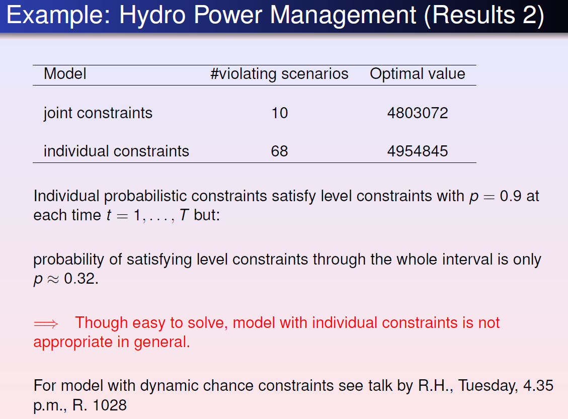
Individual chance constraints are easy to solve, however, they only guarantee that each line satisfies the constraint to a certain confidence level.
Joint chance constraint:
$$
h_i(x,\xi) \geq 0 \rightarrow P(h_i(x,\xi) \geq 0 \ (i=1,\cdots, m))\geq p \quad
$$
Joint chance constraint ensures that the constraint as a whole is satisfied to a certain confidence level, however, it is incredibly difficult to solve, even numerically.
Solving Method:
Simple case (decision and random variables can be decoupled):
chance constraints can be relaxed into deterministic constraints using probability density functions (pdf). Then, use LP or NLP to solve.
Linear ( $h$ is leaner in $\xi$ ), i.e., $P(h(x)\ge 0)\ge p$
Two types:
- separable model: $P(y(x)\ge A\xi)\ge p$
- bilinear model: $P(\Xi \cdot x \geq b) \geq p$
calculate the probability by using the probability density function (pdf) and substitute the left hand side of the constraint with a deterministic expression
- PDF :
- statistical regression (abundant data),
- interpolation and extrapolation (few data)
- Marginal distribution function (when uncertain variables has correlations)
- Feasible region depends on confidence level
- high confidence level $\rightarrow$ small feasible region
- low confidence level $\rightarrow$ larger feasible region
- can make different confidence level with important
- PDF :
Nonlinear
relax problem by transforming into deterministic NLP problem.
- Solving nonlinear chance constrained problem is difficult, because nonlinear propogation makes it hard to obtain the distribution if output variables when distribution of uncertainty is unknown.
- strategy: back-mapping
- robust optimization
- sample average approximation
- Solving nonlinear chance constrained problem is difficult, because nonlinear propogation makes it hard to obtain the distribution if output variables when distribution of uncertainty is unknown.
Complex case (decision and random variables interact and cannot decouple)
- impossible to solve.
Challenges:
Structural Challenges
Structural Property:
Probability function: $\varphi(x) :=P(h(x, \xi) \geq 0)$
set of feasible decisions: $M :=\left{x \in \mathbb{R}^{n} | \varphi(x) \geq p\right}$
Proposition ====(Upper Semicontinuity, closeness)
if $h_i$ are usc, then so is $\varphi$. Then, $M$ is closed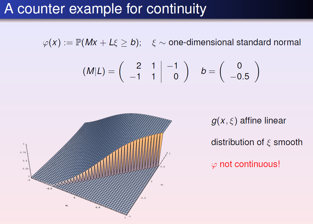
==Proposition==
if $h_i$ are continuous, and $P(h_i(x,\xi)=0)=0, \forall x \in R^n \forall i \in {1,\cdots,s}$, then $\phi$ is continuous too.==Proposition==
if $\xi$ has pdf $f_\xi$, i.e., $F_\xi(z)=\int_{-\inf}^{z} f_\xi(x) dx$, then $F_\xi$ is continuous.
==Theorem== (Wang 1985, Romisch/Schultz 1993)
If $\xi$ has a density $f_\xi$, then $F_\xi$ is Lipschitz continuous if and only if all marginal densities $f_{\xi_i}$ are essentially bounded.
==Theorem (R.H./R¨omisch 2010)==
If $\xi$ has a density $f_\xi$ such that $f^{−1/s}_\xi$ is convex, then $F_\xi$ is Lipschitz continuous
Assumption satisfied by most prominent multivariate distributions:
Gaussian, Dirichlet, t, Wishart, Gamma, lognormal, uniform
Numerical Challenges:
$$
P(y(x)\ge \xi)\ge p = P(h(\xi \leq x)\ge p) = F_\xi (h(x) \ge p)
$$
If $\xi \sim \mathcal{N}(\mu, \Sigma)$ with $\Sigma$ positive definite (regular Gaussian),
$$
\frac{\partial F_{\xi}}{\partial z_{i}}(z)=f_{\xi_{i}}\left(z_{i}\right) \cdot F_{\tilde{\xi}\left(z_{i}\right)}\left(z_{1}, \ldots, z_{i-1}, z_{i+1} \ldots, z_{s}\right) \quad(i=1, \ldots, s)
$$
Efficient method to compute $F_\xi$ (and $\nabla F_{\xi}$) :
code by A. Genz. computes Gaussian probabilities of rectangles:
$\mathbb{P}(\xi \in[a, b]) \quad\left(F_{\xi}(z)=\mathbb{P}(\xi \in(-\infty, z])\right.$
allows to consider problems with up to a few hundred random variables.
cope with more complicated models, like $\mathbb{P}(h(x) \geq A \xi) \geq p, \quad \mathbb{P}(\Xi \cdot x \geq b) \geq p$:
Compute Derivatives for Gaussian Probabilities of Rectangles
Let $\xi \sim \mathcal{N}(\mu, \Sigma)$ with $\Sigma$ positive definite. Consider a two-sided probabilistic constraint: $\mathbb{P}(\xi \in[a(x), b(x)]) \geq p$. Then, $\alpha_{\xi}(a(x), b(x)) \geq p, \quad$ where $\quad \alpha_{\xi}(a, b) :=\mathbb{P}(\xi \in[a, b])$
Partial derivatives:
Method 1:
Reduction to distribution functions, then use known gradient formula.
$$
\alpha_{\xi}(a, b)=\sum\limits_{i_{1}, \ldots, i_{s} \in{0,1}}(-1)^{\left[s+\sum_{j=1}^{s} i_{j}\right]} F_{\xi}\left(y_{i_{1}}, \ldots, y_{i_{s}}\right), \quad y_{i_{j}} :=\left{
\begin{array}{ll}
{a_{j}} & {\text { if } i_{j}=0} \
{b_{j}} & {\text { if } i_{j}=1}
\end{array}
\right.
$$
For dimension $s$, there are $2^s$ terms in the sum. Not practicable!Method 2:
$$
\alpha_{\xi}(a, b)=\mathbb{P}\left(\left(\begin{array}{c}{\xi} \ {-\xi}\end{array}\right) \leq\left(\begin{array}{c}{b} \ {-a}\end{array}\right)\right), \quad\left(\begin{array}{c}{\xi} \ {-\xi}\end{array}\right) \sim \mathcal{N}\left(\left(\begin{array}{c}{\mu} \ {-\mu}\end{array}\right),\left(\begin{array}{cc}{\Sigma} & {-\Sigma} \ {-\Sigma} & {\Sigma}\end{array}\right)\right)
$$
$\Longrightarrow$ Singular normal distribution, gradient formula not available==Proposition (Ackooij/R.H./M¨ oller/Zorgati 2010)==
Let $\xi \sim \mathcal{N}(\mu, \Sigma)$ with $\Sigma$ positive definite and $f_\xi$ the corresponding density. Then, $\frac{\partial \alpha_{\xi}}{\partial b_{i}}(a, b)=f_{\xi_{i}}\left(b_{i}\right) \alpha_{\tilde{\xi}}\left(b_{i}\right)(\tilde{a}, \tilde{b}) ; \quad \frac{\partial \alpha_{\xi}}{\partial a_{i}}(a, b)=-f_{\xi_{i}}\left(a_{i}\right) \alpha_{\tilde{\xi}}\left(a_{i}\right)(\tilde{a}, \tilde{b})$ with the tilda-quantities defined as in the gradient formula for Gaussian distribution functions.$\Longrightarrow$ Use Genz’ code to calculate $\alpha_\xi$ and $\nabla_{a, b} \alpha_{\xi}$ at a time.
Derivatives for separated model with Gaussian data:
Let $\xi \sim \mathcal{N}(\mu, \Sigma)$ with $\Sigma$ positive definite and consider the probability function:
$$
\beta_{\xi, A}(x) :=\mathbb{P}(A \xi \leq x)
$$
If the rows of $A$ are linearly independent, then put $\eta :=A \xi \sim \mathcal{N}\left(A \mu, A \Sigma A^{T}\right)$, then
$$
\Longrightarrow \quad \beta_{\xi, A}(x)=F_{\eta}(x)\quad \text{regular Gaussian distribution function}
$$
otherwise, $F_\eta$ is a singular Gaussian distribution function (gradient formula not available)
==Theorem (R.H./M¨ oller 2010, see talk by A. M¨ oller, Thursday, 3.20 p.m., R. 1020)==
$\frac{\partial \beta_{\xi, A}}{\partial x_{i}}(x)=f_{A_{i} \xi}\left(x_{i}\right) \beta_{\tilde{\xi}, \tilde{A}}(\tilde{x})$ where $\tilde{\xi} \sim \mathcal{N}\left(0, l_{s-1}\right)$ and $\tilde{A}$, $\tilde{x}$ can be calculated explicitly from $A$ and $x$.
use e.g., Deak’s code for calculating normal probabilities of convex sets.
Derivatives for bilinear model with Gaussian data
probability function: $\gamma(x) :=\mathbb{P}(\Xi x \leq a)$ with normally distributed $(m,s)$ coefficient matrix. Let $\xi_i$ be the $i$th row of $\Xi$\
$$
\begin{array}{rCl}
\gamma(x) &=F_{\eta}(a) \ \nabla \gamma(x) &=\sum_{i=1}^{m} \frac{\partial F_{\eta}}{\partial z_{i}}(\beta(x)) \nabla \beta_{i}(x)+\sum_{i, j=1}^{m} \frac{\partial^{2} F_{\eta}}{\partial z_{i} \partial z_{j}}(\beta(x)) \nabla R_{i j}(x)
\end{array}
$$
$$
\begin{aligned} \eta & \sim \mathcal{N}(0, R(x)) \ \mu(x) &=\left(\mathbb{E} \xi_{i}^{T} x\right){i=1}^{m} \ \Sigma(x) &=\left(x^{T} \operatorname{Cov}\left(\xi{i}, \xi_{j}\right) x\right){i, j=1}^{m} \ D(x) &=\operatorname{diag}\left(\Sigma{i i}^{-1 / 2}(x)\right)_{i=1}^{m} \ R(x) &=D(x) \Sigma(x) D(x) \ \beta(x) &=D(x)(a-\mu(x)) \end{aligned}
$$
e.g. hold constraints and gradients constant while calculating probabilities. [No closed-form analytical representation of probabilities]
Convexity Challenges
$$
P(y(x)\ge \xi)\ge p = P(h(\xi \leq x)\ge p) = F_\xi (h(x) \ge p)
$$
Global optimization: if the optimization problem is convex, the local optimum is global optimum; otherwise, methods such as McCormick Envelope Approximation should be used.
if $F_\xi (h(x) \ge p)$ is concave, the optimization problem is convex.
Sufficient:
- components $h_j$ concave: e.g., $h$ is a linear mapping
- $F_\xi $ increasing: automatic (distribution function)
- $F_\xi$ concave: Never, because pdf bounded by 0 and 1.
If exist a strictly increasing function $\varphi: \mathbb{R}{+} \rightarrow \mathbb{R} $ such that $\varphi \circ F{\xi}$ is concave:
i.e., $F_\xi (h(x) \ge p) \iff \varphi(F_\xi (h(x)) \ge \varphi(p)$.
then, $\underbrace{\varphi \circ F_{\xi}}_{\text {increasing } \atop \text { concave }} \circ h$ is concave if the components $h_i$ are concave
potential candidates: $\varphi = \log$, $\varphi=-(\cdot)^{-n}$

==Theorem (Pr´ekopa 1973 )==
Log-concavity of the density implies log-concavity of the distribution function.example log-concave distribution: Normal, Gaussian, Dirichlet, Student, lognormal, Gamma, uniform, Wishart
Separable model:
==Corollary (Convexity in the separable model)==
Consider the feasible set $M := {x \in \mathbb{R}^n | P(A\xi \leq h(x)) \geq p}$. Let $\xi$ have a density $f_\xi$ such that $\log f_\xi$ is concave and let the $h_i$ be concave (e.g., $h$ linear). Then, $M$ is convex for any $p\in[0, 1]$.Bilinear model:
feasible set $M :=\left{x \in \mathbb{R}^{n} | \mathbb{P}(\Xi x \leq a) \geq p\right}$
==Theorem (Van de Panne/Popp, Kataoka 1963, Kan 2002, Lagoa/Sznaier 2005)==
Let $\Xi$ have one row only which has an elliptically symmetric or log-concave symmetric distribution (e.g., Gaussian). Then, $M$ is convex for $p\ge 0.5$.
==Theorem (R.H./Strugarek 2008)==
Let the rows $\xi_i$ of $\Xi$ be Gaussian according to $\xi_i \sim \mathcal{N}(\mu_i,\Sigma_i)$. If the $\xi_i$ are pairwise independent, then $M$ is convex for $p > \Phi(\max{\sqrt{3},\tao}), where
- $\Phi =$ 1-dimensional standard normal distribution function
- $\tau=\max {i} \lambda{\max }^{(i)}\left[\lambda_{\min }^{(i)}\right]^{-3 / 2}\left|\mu_{i}\right|$
-$\lambda_{\max }^{(i)}, \lambda_{\min }^{(i)} :=$ largest and smallest eigenvalue of $\Sigma_i$.
Moreover, $M$ is compact for $p>\min {i} \Phi\left(\left|\mu{i}\right|{\Sigma{i}^{-1}}\right)$
A challenging issue comes in when the distribution is uniform or normal with independent components, since these may lack strong log concavity in certain circumstances. Furthermore, it should be noted that the Student’s t-distribution, the Cauchy distribution, the Pareto distribution, and the log-normal distribution are not log concave.
Stability Challenges
Distribution of $\xi$ rarely known $\Longrightarrow$ Approximation by some $\eta$ $\Longrightarrow$ Stability?
==Theorem (R.H./W.R¨omisch 2004)==
- $f$ convex, $C$ convex, closed, $\xi$ has log-concave density
- \Psi(\xi)$ nonempty and bounded
- $\exists x \in C : \quad \mathbb{P}(\xi \leq A x)>p$ (Slater point)
Then, $\Psi$ is upper semicontinuous at $\xi$:
$$
\Psi(\eta) \subseteq \Psi(\xi)+\varepsilon \mathbb{B} \quad \text { for } \quad \sup {z \in \mathbb{R}^{s}}\left|F{\xi}(z)-F_{\eta}(z)\right|<\delta
$$
If in addition - $f$ convex-quadratic, $C$ polyhedron,
- $\xi$ has strongly log-concave distribution function,
then $\Psi$ is locally Hausdorff-Holder continuous at $\xi$:
$$
\left.d_{\text {Haus }}(\psi(\eta), \psi(\xi)) \leq L \sqrt{\sup {z \in \mathbb{R}^{s}}\left|F{\xi}(z)-F_{\eta}(z)\right|} \quad \text { (locally around } \xi\right)
$$
pdf is nor precise, most is approximation.
- slight changes in distribution may cause major changes to optimum
- if assumed distribution is slightly different from actual distribution, not stable.
- In order to achieve Hölder- or Lipschitz stability one has to impose further structural conditions, such as strong log-concavity, strict complementarity, and C1,1-differentiability.
Applications
Engineering:
UGV, UAV: Optimal Navigation and Reliable Obstacles Avoidance
System description:
$$
\begin{aligned}
\dot x & = f(x,u,\xi)\
0 & = g(x,u,\xi)
\end{aligned}
$$
$\xi$ may be:
- random obstacles
- sensor measurement errors
- state generated errors
Probability density function of these variables are estimated based on previous data. and formulated into chance constraints.
Based on these constraints, unmanned vehicles can travel through a specific region with the shortest distance while avoiding random obstacles at a high confidence level.2
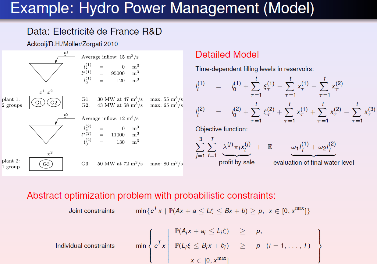
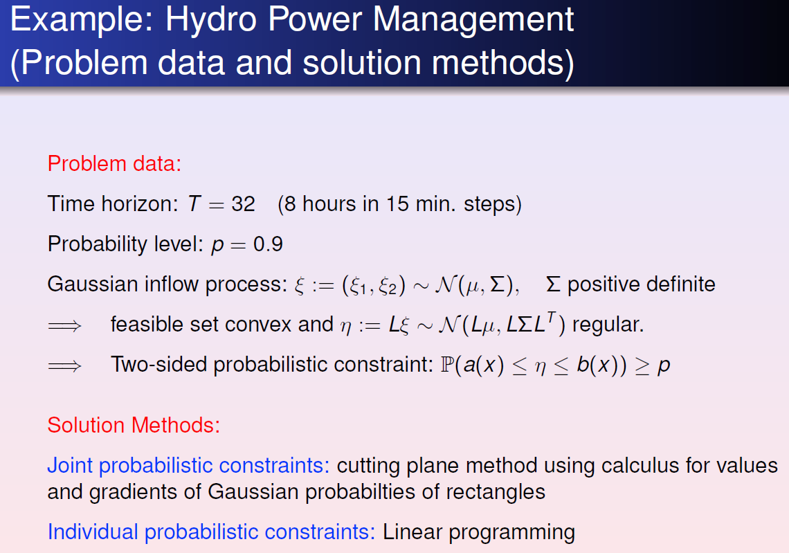
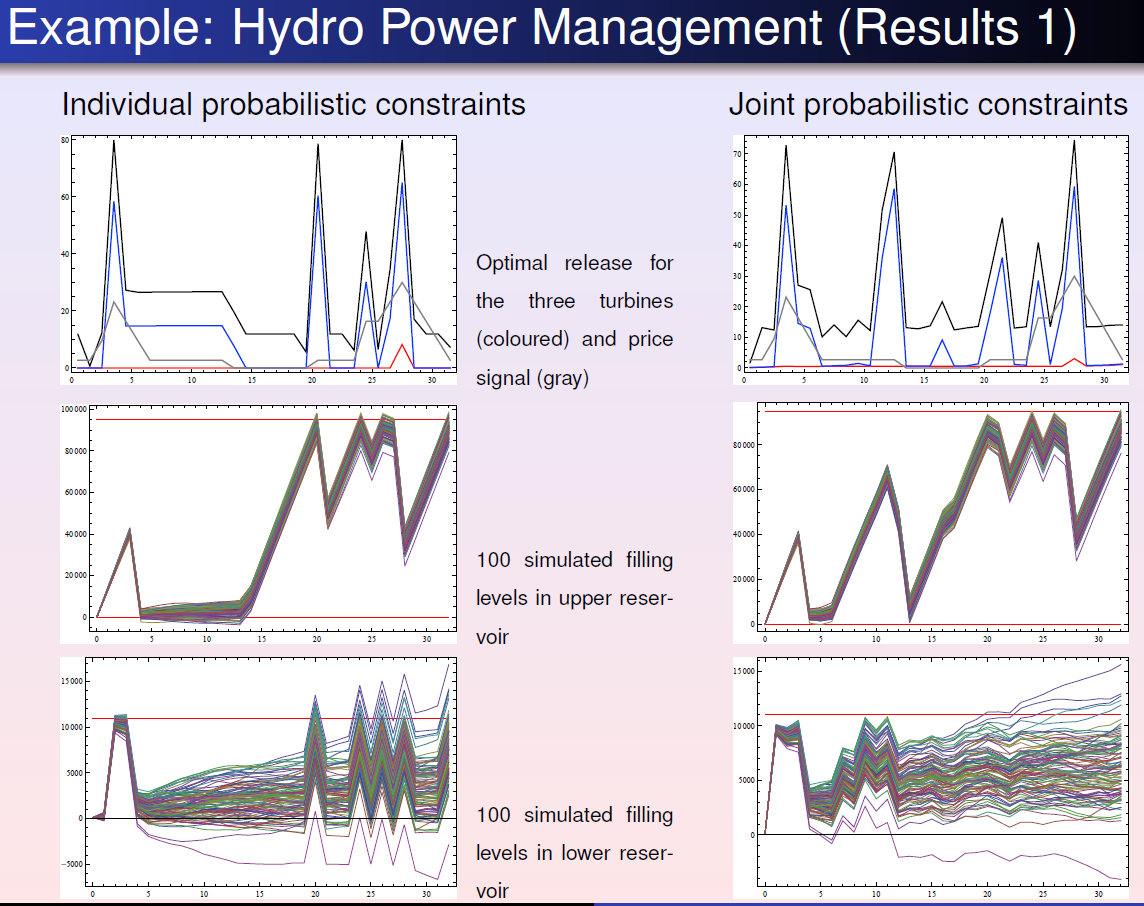
Power system management:
Risk management
Conclusion
The chance-constraint method is a great way to solve optimization problems due to its robustness. It allows one to set a desired confidence level and take into account trade-off between two or more objectives. However, it can be extremely difficult to solve. Probability density functions are often difficult to formulate, especially for the nonlinear problems. Issues with convexity and stability of these questions mean that small deviations from the actual density function could cause major changes in the optimal solution. Further complications are added when the variables with and without uncertainty can not be decoupled. Due to these complications, there’s no single approach to solving chance-constraint problems. Though the most common approach to simple questions is to transform the chance constraints into deterministic functions by decoupling the variables with and without uncertainty and using probability density functions.
This approach has many applications in the engineering field and the finance field. Namely, it is widely used in energy management, risk management, and more recently, determination of production level, performance of industrial robots, and performance of unmanned vehicle. A lot of research in the area focuses on solving nonlinear dynamic questions with chance constraints.