3. RL algorithms

DQN and variants
DQN
Value: (state, reward, state_new)
$Q(s,a)$ 与当前得到的reward 和 $Q(s’,a)$有关。
价值函数近似:
$Q(s,a)=f(s,a)$, here, $f$ can be represented by NN. –> $Q(s,a)=f(s,a,w)$ where $w$ is hte parameter of NN.
How to get the state_new? we trial and error –> have state_new from previous experiences.
流程;
首先环境会给出一个obs,智能体根据值函数网络得到关于这个obs的所有Q(s,a),然后利用$ϵ$−greedy选择action并做出决策,环境接收到此action后会给出一个奖励Rew及下一个obs。这是一个step。此时我们根据Rew去更新值函数网络的参数。接着进入下一个step。如此循环下去,直到我们训练出了一个好的值函数网络。
Q value的更新依靠$Q_{target}$:(利用reward和Q计算出来的目标Q value), $R_{t+1}+\gamma\max_a Q(s_{t+1},a)$.
所以,我们把$Q_{target}$作为标签,使$Q$趋近于$Q_{target}$.
所以,loss function is $\ell(w)=\mathbb{E}[\underbrace{r+\gamma\max_{a’}Q(s’,a’,w) }{Q{target}}- Q(s,a,w)]$.
具体流程:
每次只要传入一组(s,a,r,s’),即当前所处状态s,当前选择的动作a,做出动作a后获得的奖励r,以及做出动作a后转移到的下一状态s’。这四个值都可以在模拟一局游戏时取到,而且每模拟一局游戏能取到非常多组数据。在论文中作者提出了经验回放(experience replay)的采集数据方法,即事先采样足够多组的数据放入一个固定容量的经验池中,然后每次训练时从该经验池中随机取出一个batch的数据进行梯度下降更新参数。值得注意的是这一个batch的数据训练完成后是放回经验池的,也就是说下次训练时是可以复用的。只有当产生新的数据时,才会更新经验池。当一轮训练完成,更新完模型参数后,再根据该模型提供的策略进行模拟游戏,产生新的数据并放入经验池中,由于该经验池是有最大容量的,所以最早的一些数据会被新的数据替代。像这样每玩几局游戏训练一次(玩游戏的同时其实是在更新训练数据),极大地提升了训练的效率。此外,为了更加稳定地训练模型,作者提出了固定target值的思想,具体做法是复制一个和原本Q网络一模一样的target-Q网络用于计算target值,使得target-Q网络的参数在一定时间段内保持固定不变,在这段时间内用梯度下降训练Q网络。然后阶段性地根据Q网络学习完后的参数更新这个target-Q网络(就是把Q网络的参数再复制过去)。

Q-Learning的target是 $R_{t+1}+γ\max_{a′}Q(S_{t+1},a′)$。它使用 $ϵ$−greedy策略来生成action $a_{t+1}$,但用来计算target的action却不一定是$a_{t+1}$,而是使得$Q(S_{t+1},a)$最大的action。这种产生行为的策略和进行评估的策略不一样的方法称为Off-policy方法。对于Q-Learning来说,产生行为的策略是$$ϵ$$−greedy,而进行评估的策略是greedy。$Q(s,a)\leftarrow Q(s,a)+\alpha(R+\gamma\max_{a’}Q(s’,a’)-Q(s,a))$
SarSa中使用$ϵ$−greedy策略生成action $a_{t+1}$,随即又用 $a_{t+1}$处对应的值函数来计算target,更新上一步的值函数。这种学习方式又称为On-policy。$Q(s,a)\leftarrow Q(s,a)+\alpha(R+\gamma Q(s’,a’)-Q(s,a))$
Double DQN
DDQN的模型结构基本和DQN的模型结构一模一样,唯一不同的就是它们的目标函数。
$$
Q^{DQN}{target}(s,a) = R{t+1} + \gamma \max_aQ(s’,a;\hat\theta)\
Q^{DoubleDQN}{target}(s,a) = R{t+1} + \gamma Q(s’, \operatorname{argmax}_a Q(s’,a;\theta),\hat\theta)
$$
这两个target函数的区别在于DoubleDQN的最优动作选择是根据当前正在更新的Q网络的参数 $\theta_t$,而DQN中的最优动作选择是根据target-Q网络的参数$\hat\theta_t$。这样做的原因是传统的DQN通常会高估Q值的大小(overestimation)。
而DDQN由于每次选择的根据是当前Q网络的参数,并不是像DQN那样根据target-Q的参数,所以当计算target值时是会比原来小一点的。(因为计算target值时要通过target-Q网络,在DQN中原本是根据target-Q的参数选择其中Q值最大的action,而现在用DDQN更换了选择以后计算出的Q值一定是小于或等于原来的Q值的)这样在一定程度上降低了overestimation,使得Q值更加接近真实值。
Dueling DQN

把Q function拆分为state function和advantage function :$Q(s,a;\theta, \alpha, \beta) = V(s;\theta, \beta)+A(s,a;\theta,\alpha)$, 式中,$V(s;\theta, \beta)$是state function,输出一个标量,$A(s,a;\theta,\alpha)$是advantage function,输出一个矢量,矢量长度等于动作空间大小; $\theta$指网络卷积层的参数; $\alpha$和$\beta$分别是2个分支的全连接层的参数
$$
V^\pi(s) = \mathbb E_{a\sim\pi(s)}[Q^\pi(s,a)] \
A^\pi(s,a) = Q^\pi(s,a) - V^\pi(s)
$$
V代表了在当前状态s下,Q值的平均期望(综合考虑了所有可选动作)。A代表了在选择动作a时Q值超出期望值的多少。两者相加就是实际的Q(s,a)。所以这样设计模型就是为了让神经网络对给定的s有一个基本的判断,在这个基础上再根据不同的action进行修正。但是按照上述想法直接训练是有问题的,问题就在于若神经网络把V训练成固定值0后,就相当于普通的DQN网络了,因为此时的A值就是Q值。所以我们需要给我们的神经网络加一个约束条件,让所有动作对应的A值之和为零,使得训练出的V值是所有n个Q值的平均值(n代表可选择的动作个数)。
$$
Q(s,a;\theta, \alpha, \beta) = V(s;\theta, \beta)+ (A(s,a;\theta,\alpha) - \frac{1}{|\mathcal A|} \sum_{a’}A(s,a’;\theta,\alpha)
$$
式中,里括号中的部分其实就是之前说的A值,公式里的$|\mathcal A|$代表了可选择动作的个数。可以明显看出若把|A|个动作对应的括号中的部分相加,它们的和为零。所以问题就转化为利用神经网络求上述公式中的V(s; \theta,\beta)与A(s,a; \theta, \alpha)。其中V(s; θ \theta θ, β \beta β)就是前文所提到的V值,而A(s,a; θ \theta θ, α \alpha α)和前文所提到的广义上的A值其实不一样,但可以通过A(s,a; θ \theta θ, α \alpha α)计算出A值。
Summary

- Double DQN:目的是减少因为max Q值计算带来的计算偏差,或者称为过度估计(over estimation)问题,用当前的Q网络来选择动作,用目标Q网络来计算目标Q。
- Prioritised replay:也就是优先经验的意思。优先级采用目标Q值与当前Q值的差值来表示。优先级高,那么采样的概率就高。
- Dueling Network:将Q网络分成两个通道,一个输出V,一个输出A,最后再合起来得到Qr。
Policy-based method
Policy gradient
一个角度来看
State-value function: $V_\pi(s_t) = \mathbb E_A [Q_\pi(s_t, A)] = \sum_a \pi(a|s_t) Q_\pi(s_t,a)$
通过state-value function的定义引出用策略网络来近似策略函数
Approximate the state-value function:
- Approximate policy function $\pi(a|s_t)$ by policy network $\pi(a|s_t;\theta)$.
- Approximate value function $V_\pi(s_t)$ by $V_\pi(s_t) = \sum_a \pi(a|s_t;\theta) Q_\pi(s_t,a)$.
用评价函数$L(\theta)$来评价策略的好坏,进而用策略梯度进行求解
learn $\theta$ that maximizes $L(\theta)=\mathbb E_S[V(S;\theta)]$
How to improve $\theta$?
observe state $s$.
update policy by $\theta \leftarrow \theta + \beta \underbrace{ \frac{\partial V(s;\theta)}{\partial \theta}}{policy\ gradient}$.
$$
\begin{array}{rCl}
\frac{\partial V(s;\theta)}{\partial \theta}
&=& \frac{\partial \sum_a \pi(a|s;\theta) Q_\pi(s,a)}{\partial \theta} \
&=& \sum_a \frac{\partial \pi(a|s;\theta) Q_\pi(s,a)}{\partial \theta} \
&=& \sum_a \frac{\partial \pi(a|s;\theta) }{\partial \theta} Q_\pi(s,a) \quad \text{assume $Q{\pi}$ is independent of $\theta$} \
&=& \sum_a \pi(a|s;\theta) ; \frac{\partial \log \pi(a|s;\theta) }{\partial \theta} Q_\pi(s,a) \
&=& \mathbb E_{A\sim\pi(\cdot|s,\theta)} \left[ \frac{\partial \log \pi(a|s;\theta) }{\partial \theta} Q_\pi(s,a) \right]
\end{array}
$$
Thus, we have two forms of policy gradient:
$$
\begin{array}{rCl}
\text{Form 1: } &\quad& \frac{\partial V(s;\theta)}{\partial \theta} = \sum_a \frac{\partial \pi(a|s;\theta) }{\partial \theta} Q_\pi(s,a) \
\text{Form 2: } &\quad& \frac{\partial V(s;\theta)}{\partial \theta} = \mathbb E_{A\sim\pi(\cdot|s,\theta)} \left[ \frac{\partial \log \pi(a|s;\theta) }{\partial \theta} Q_\pi(s,a) \right]
\end{array}
$$
Case 1 (discrete actions) –> Form 1
Calculate $f(a,\theta) = \frac{\partial \pi(a|s;\theta) }{\partial \theta} Q_\pi(s,a)$ for every acton $a\in \mathcal A$.
Policy gradient: $\frac{\partial V(s;\theta)}{\partial \theta} = \sum_a f(a,\theta)$
if $|\mathcal A|$ is vast, this approach is costly.
Case 2 (continuous actions) –> Form 2
在求连续动作时,需要求定积分,这很难。一般采用Monte-Carlo近似的方法求出期望函数的无偏估计。(对于离散动作,这种方法也适用)。
- Randomly sample an action $\hat a$ according to the PDF $\pi(\cdot|s;\theta)$
- Calculate $g(\hat a, \theta) = \frac{\partial \log \pi(\hat a|s;\theta) }{\partial \theta} Q_\pi(s, \hat a)$
- Use $g(\hat a, \theta)$ as an approximation to the policy gradient $\frac{\partial V(s;\theta)}{\partial \theta}$.
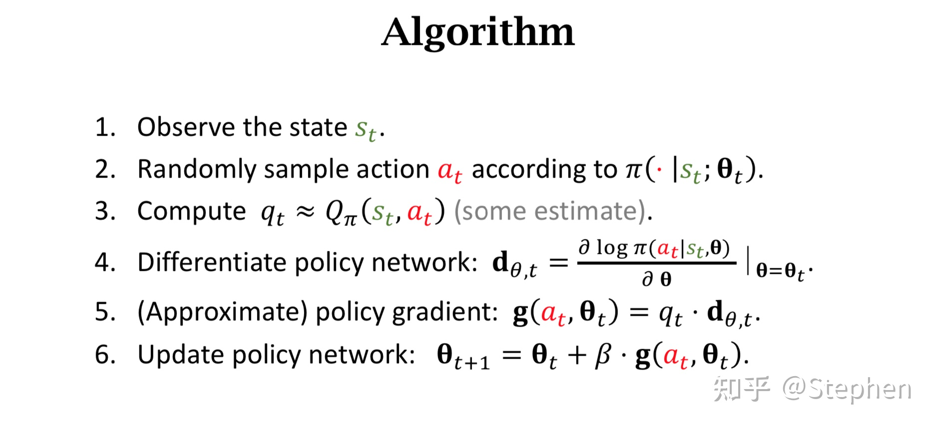
Algorithm:
Pros and Cons:
- Advantages:
- efficient in high-dimensional or continuous action spaces (output actions probability)
- can learn stochastic policies
- better convergence properties
- Disadvantages:
- typocally converge to a local rather global optimum
- evaluating a policy is typically inefficient and high variance
- Advantages:
遗留的问题: How to calculate $q_t$???
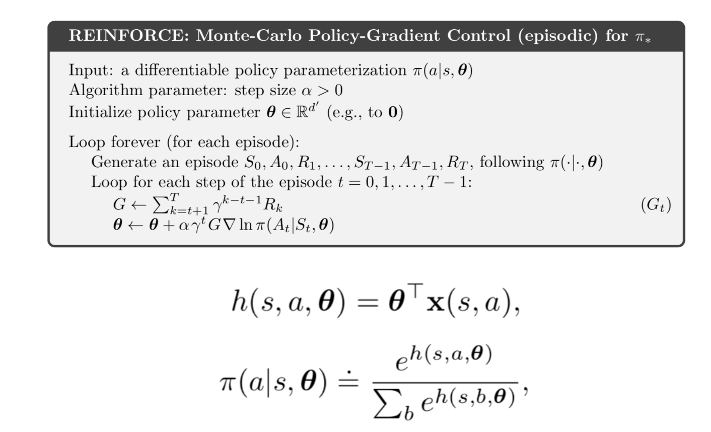
Method 1: Reinforce
- Play the game to the end and generate the trajectry <$s_1, a_1, r_1, s_2, a_2, r_2, \cdots, S_T, a_T, r_T$>
- Compute the discounted return $G_t = \sum_{k=t}^T \gamma^{k-t} r_k$ for all $t$.
- Since $Q_\pi(s_t,a_t) = \mathbb E[G_t]$, we can use $u_t$ to approximate $Q_\pi(s_t,a_t)$.
- –> $q_t = u_t$.
Method 2: Actor-Critic
- approximate $Q_\pi$ using a neural network.
另一个角度来看
Loss: $L(\theta) = \mathbb E(r1 + \gamma r2 + \gamma^2r_3 + \cdots | \pi(,\theta))$ , 所有带衰减reward的累计期望
如何能够计算出损失函数关于参数的梯度(也就是策略梯度)$\nabla_\theta L(\theta)$:
- 对于一个策略网络,输入state,输出action的概率。然后execute action, 得到reward。
- 如果某一个动作得到reward多,使其出现的概率增大,如果某一个动作得到的reward少,使其出现的概率减小。
- 如果能够构造一个好的动作评判指标,来判断一个动作的好与坏,那么我们就可以通过改变动作的出现概率来优化策略!
–> 使用log likelihood $\log \pi(a|s,\theta)$, 且给定critic metric是$f(s,a)$.
–> Loss:$L(\theta) = \sum \log \pi(a|s,\theta) f(s,a)$
Parametrise the policy: $\pi_\theta(s,a)=\mathbb P \left[a|s,\theta\right]$.
$$
\nabla_\theta \pi_\theta(s,a) = \pi_\theta(s,a) \frac{\nabla_\theta \pi_\theta(s,a)}{\pi_\theta(s,a)} = \underbrace{\pi_\theta(s,a)}{policy} \underbrace{\nabla_\theta \log \pi_\theta(s,a)}{score\ function}
$$
- softmax policy: [discrete action space]
- weighting actions using linear combination of features $\phi(s,a)^\top\theta$
- probability of action is proportional to exponentiated weight $\pi_\theta(s,a) \propto e^{\phi(s,a)^\top \theta}$
- The score function is $\nabla_\theta \log \pi_\theta(s,a) = \phi(s,a) - \mathbb E_{\pi_\theta} [\phi(s,\cdot)]$
- Gaussian policy: [continuous action space]
- mean is linear combination of state feature $\mu(s) = \phi(s)^\top \theta$
- variance is fixed $\sigma^2$ or parameterised
- policy is Gaussian $a\sim\mathcal N(\mu(s),\sigma^2)$
- the score function is $\nabla_\theta \log \pi_\theta(s,a) = \frac{(a-\mu(s))\phi(s)}{\sigma^2}$
缺点:
require full episodes
high gradients variance. $\nabla L \simeq \mathbb E [Q(s,a) \nabla \log \pi(a|s)]$ which is proportional to the discounted reward from the given state.
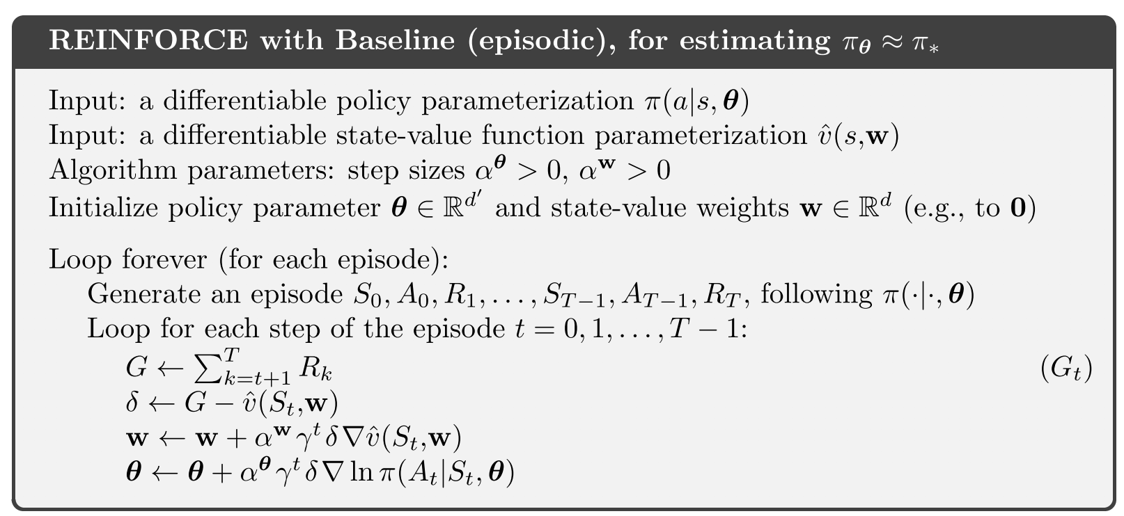
–> add baseline from $Q$, which can be :
- some constant value (mean of the discounted rewards)
- moving average of discouted rewards
- the value of the state $V(s)$
Exploration. entropy 表征uncertainty。
为避免local optimum,substract entropy from the loss function and punish the entropy to be too certain.
Correlation between samples.
Actor-critic and Variants
Actor-critic
reduce the variance of the gradient (由于很难infinite交互,期望与真实有差异,会带来较大的variance)
actor-critic用一个独立模型估计轨迹的长期return,而不是直接使用轨迹的真实return。(类似于基于模型的Q-Learning 算法,在估计时使用模型估计轨迹价值,在更新时利用轨迹的回报得到目标价值,然后将模型的估计值和目标值进行比较,从而改进模型。)
$\nabla_\theta L(\theta) = \frac{1}{N} \sum_{i=1}^N\sum_{t=0}^T \left[\nabla_\theta \log \pi_\theta (a_{i,t}|s_{i,t}) \left(\sum_{t’=t}^{T}r(s_{i,t’},a_{i,t’}) - b_i \right)\right]$
方案:
- 使用策略梯度法: $\sum_{t’=t}^{T}r(s_{i,t’},a_{i,t’}) - b_i$
- 使用状态值函数估计轨迹的return: $q(s,a)$
- 使用优势函数估计轨迹的return: $A(s,a) = q(s,a) - V(s)$
- 使用TD-Error估计轨迹的return: $r(s,a) + q(s) - q(s’)$ [只需要算一个价值函数V,V函数和动作无关,可以用来计算Q和A]
Evaluation for value function
- Monte Carlo (用整条轨迹计算)
- $V^\pi(s_t) \approx \sum_{t’=t}^T r(s_{t’}, a_{t’})$
- Training data: $\left{ \left(s_{i,t}, \underbrace{\sum_{t’=t}^T r(s_{t’}, a_{t’})}{y{i,t}}\right) \right}$
- Loss: $L = \frac{1}{2} \sum_i | \hat V^\pi(s_i) - y_i |^2$
- TD (bootstrap):
- Training data: $\left{ \left(s_{i,t}, \underbrace{ r(s_{i,t}, a_{i,t})+ \hat V^\pi_\phi (s_{i,t+1})}{y{i,t}}\right) \right}$
- 引入了适当的bias, –> 减小variance
- Monte Carlo (用整条轨迹计算)
Actor Critic Design Decisions
- 用两个网络分别去拟合Actor网络和Critic网络
- 优势是容易训练且稳定;缺点是没有共享feature,导致参数量增大,计算量也增大
- 用同一个网络去拟合:
- 解决了两个网络的优势,但是有可能会出现两个部分冲突的问题
- 用两个网络分别去拟合Actor网络和Critic网络
Actor-Critic方法和Policy Gradient方法各有优劣:Actor-Critic方法方差小但是有偏,Policy-Gradient无偏但是方差大:
Actor-critic: $\nabla_\theta L(\theta) = \frac{1}{N} \sum_{i=1}^N\sum_{t=0}^T \left[\nabla_\theta \log \pi_\theta (a_{i,t}|s_{i,t}) \left(r(s_{i,t},a_{i,t}) + \gamma\hat V^\pi_\phi(s_{i,t+1}) - \hat V^\pi_\phi(s_{i,t}) - b_i \right)\right]$
lower variance with bias
Policy graddient: $\nabla_\theta L(\theta) = \frac{1}{N} \sum_{i=1}^N\sum_{t=0}^T \left[\nabla_\theta \log \pi_\theta (a_{i,t}|s_{i,t}) \left(\sum_{t’=t}^{T}\gamma^{t’-t}r(s_{i,t’},a_{i,t’}) - b_i \right)\right]$
no bias with higher variace (because use single sample estimate)
So, 结合两种方法,–> no bias with low variance (because baseline is close to reward)
$$
\nabla_\theta L(\theta) = \frac{1}{N} \sum_{i=1}^N\sum_{t=0}^T \left[\nabla_\theta \log \pi_\theta (a_{i,t}|s_{i,t}) \left(\sum_{t’=t}^{T} \gamma^{t’-t}r(s_{i,t’},a_{i,t’}) - \hat V_\phi^\pi(s_{i,t}) \right)\right]
$$
如果用整条轨迹,或者仅仅一个step,都有缺点 –> 折中一下 –> n-step
$$
\nabla_\theta L(\theta) = \frac{1}{N} \sum_{i=1}^N\sum_{t=0}^T \left[\nabla_\theta \log \pi_\theta (a_{i,t}|s_{i,t}) \left(\sum_{t’=t}^{t+n} \gamma^{t’-t}r(s_{i,t’},a_{i,t’}) - \hat V_\phi^\pi(s_{i,t}) + \gamma^n \hat V_\phi^\pi(s_{i,t+n})\right)\right]
$$
随着AC的run,networks变得越来越确定optimum value,sigma变得越来越小,越来越倾向于exploiting,而不是exploring
A2C
A3C


Parallel actor-learners have a stabilizing effect on training allowing many methods (DQN, n-step Sarsa, AC) to successfully train NN.
与memory replay不同,A3C允许多个agents独立play on separate environments. Each environment is in CPU.
global optimizer and global actor-critic. each agent interact environments in separate thread. Agents reach terminal state –> gradient descent on global optimizer
Pseudocode:

具体实现:
使用torch的multiprocessing模块来生成多个trainer进程,每个进程里都会有一个player与环境交互并采集样本,定期利用buffer中的数据进行梯度更新。为了保证异步更新的有效性,在main进程里实例化了一个share model (global_actor_critic),并且通过global的optimizer来对异步收集的梯度进行优化。
1 | global_actor_critic = Agent(input_dims=input_dims, n_actions=n_actions, gamma=GAMMA) # global network |
在每个train进程中,每个agent需要定期地和global_actor_critic进行同步,从而保证整体优化的方向一致。
1 | self.local_actor_critic.actor_critic.load_state_dict(self.global_actor_critic.actor_critic.state_dict()) |
因此,我们可以得到train进程使用的是需要优化的目标策略,并且该模型是被所有进程所共享的,在global optimizer中可以实现share model (global_actor_critic)的更新。但是,在train进程中,每个agent的model是单独实例化的,因此并不和share model共享内存空间,只是会定期地通过load_state_dict()来获取共享模型的参数。player和环境交互采样得到的trajectory用于计算policy loss和value loss,通过backward获得model的梯度。然而这些梯度都是train进程player model上的,并不在share model中,所以必须要有某个机制来进行同步。因此,可以以下方法实现:
1 | for local_param, global_param in zip(self.local_actor_critic.actor_critic.parameters(), self.global_actor_critic.actor_critic.parameters()): |
注意,这里的=赋值是一个浅拷贝,因此是共享地址的,也就是share model的参数的梯度和player model参数的梯度共享一个内存空间,那么自然梯度就完成了同步。
Actor-Critic based methods
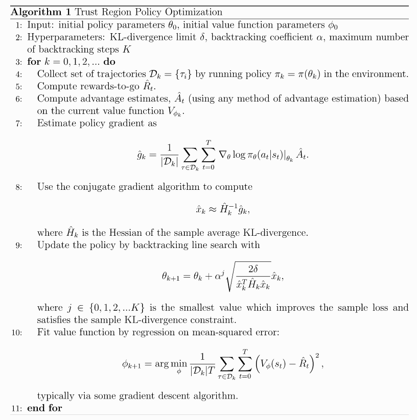
TRPO
Property:
- On-policy
- can be used for environments with either discrete or continuous action spaces.
- supports parallelization
policy update: $\theta = \theta_{old} + \alpha \nabla_\theta J$.
更新步长$\alpha$非常重要,当步长不合适时,更新的参数所对应的策略是一个更不好的策略,当利用这个更不好的策略进行采样学习时,再次更新的参数会更差,因此很容易导致越学越差,最后崩溃。选择合适的步长$\alpha$使得新的回报函数的值单调递增。
回报函数: $\eta(\tilde\pi)=E_{\tau \mid \tilde\pi}\left[\sum_{t=0}^{\infty} \gamma^{t}\left(r\left(s_{t}\right)\right)\right]$.
如果可以将新的策略所对应的回报函数$\eta(\tilde\pi)$分解成旧的策略所对应的回报函数$$\eta(\pi)$$+其他项。只要新的策略所对应的其他项大于等于零,那么新的策略就能保证回报函数单调不减。
$$
\eta(\tilde\pi)=\eta(\pi)+E_{s_{0}, a_{0}, \cdots \sim\eta(\tilde\pi)}\left[\sum_{t=0}^{\infty} \gamma^{t} A_{\pi}\left(s_{t}, a_{t}\right)\right]
$$
其中,$\tilde\pi$ 和 $\pi$ 分别表示新策略和旧策略,$\begin{array}{c}
A_{\pi}(s, a)=Q_{\pi}(s, a)-V_{\pi}(s)
=E_{s^{\prime} \sim P\left(s^{\prime} \mid s, a\right)}\left[r(s)+\gamma V^{\pi}\left(s^{\prime}\right)-V^{\pi}(s)\right]
\end{array}$.
Proof:
$$
\begin{array}{rcl}
&& E_{\tau \mid \tilde{\pi}}\left[\sum\limits_{t=0}^{\infty} \gamma^{t} A_{\pi}\left(s_{t}, a_{t}\right)\right] \
&=& E_{\tau \mid \tilde{\pi}}\left[\sum\limits_{t=0}^{\infty} \gamma^{t}\left(r(s)+\gamma V^{\pi}\left(s_{t+1}\right)-V^{\pi}\left(s_{t}\right)\right)\right] \
&=& E_{\tau \mid \tilde{\pi}}\left[\sum\limits_{t=0}^{\infty} \gamma^{t}\left(r\left(s_{t}\right)\right)+\sum\limits_{t=0}^{\infty} \gamma^{t}\left(\gamma V^{\pi}\left(s_{t+1}\right)-V^{\pi}\left(s_{t}\right)\right)\right] \
&=& E_{\tau \mid \tilde{\pi}}\left[\sum\limits_{t=0}^{\infty} \gamma^{t}\left(r\left(s_{t}\right)\right)\right]+E_{s_{0}}\left[-V^{\pi}\left(s_{0}\right)\right] \
&=&\eta(\tilde{\pi})-\eta(\pi)
\end{array}
$$
因此,可以转化为
$$
\begin{array}{rCl}
\eta(\tilde{\pi}) &=&
\eta(\pi)+\sum\limits_{t=0}^{\infty} \sum\limits_{s} P\left(s_{t}=s \mid \tilde{\pi}\right)\sum\limits_{a} \tilde{\pi}(a \mid s) \gamma^{t} A_{\pi}(s, a) \
&=& \eta(\pi)+\sum\limits_{s} \rho_{\tilde{\pi}}(s) \sum\limits_{a} \tilde{\pi}(a \mid s) A^{\pi}(s, a)
\end{array}
$$
其中,$\rho_{\pi}(s)=P\left(s_{0}=s\right)+\gamma P\left(s_{1}=s\right)+\gamma^{2} P\left(s_{2}=s\right)+\cdots$表示discounted visitation frequencies。 此时状态$s$的分布对新策略$\tilde\pi$严重依赖。
用旧策略$\pi$的状态分布来代替新策略$\tilde\pi$的状态分布,surrogate loss function is
$$
\begin{array}{rCl}
L_\pi(\tilde{\pi})
&=& \eta(\pi)+\sum\limits_{s} \rho_(s) \sum\limits_{a} \tilde{\pi}(a \mid s) A^{\pi}(s, a)
\end{array}
$$
此时,产生动作$a$是基于新的策略$\tilde\pi$,但新策略$\tilde\pi$的参数$\theta$是未知的,无法应用。
利用重要性采样对动作分布进行处理:
$$
\sum_{a} \tilde{\pi}{\theta}\left(a \mid s{n}\right) A_{\theta_{\text {old}}}\left(s_{n}, a\right)=E_{a \sim q}\left[\frac{\tilde{\pi}{\theta}\left(a \mid s{n}\right)}{q\left(a \mid s_{n}\right)} A_{\theta_{\text{old}}}\left(s_{n}, a\right)\right]
$$
surrogate loss function变为:
$$
\sum_{a} \tilde{\pi}{\theta}\left(a \mid s{n}\right) A_{\theta_{\text {old}}}\left(s_{n}, a\right)=E_{a \sim q}\left[\frac{\tilde{\pi}{\theta}\left(a \mid s{n}\right)}{q\left(a \mid s_{n}\right)} A_{\theta_{\text{old}}}\left(s_{n}, a\right)\right]
$$
比较该surrogate loss function $L_\pi(\tilde\pi)$ 和 $\eta(\tilde\pi)$:
$$
\begin{aligned}
L_{\pi_{\theta_{o l d}}}\left(\pi_{\theta_{o l d}}\right) &=\eta\left(\pi_{\theta_{o l d}}\right) \
\left.\nabla_{\theta} L_{\pi_{\theta_{o l d}}}\left(\pi_{\theta}\right)\right|{\theta=\theta{o l d}} &=\left.\nabla_{\theta} \eta\left(\pi_{\theta}\right)\right|{\theta=\theta{o l d}}
\end{aligned}
$$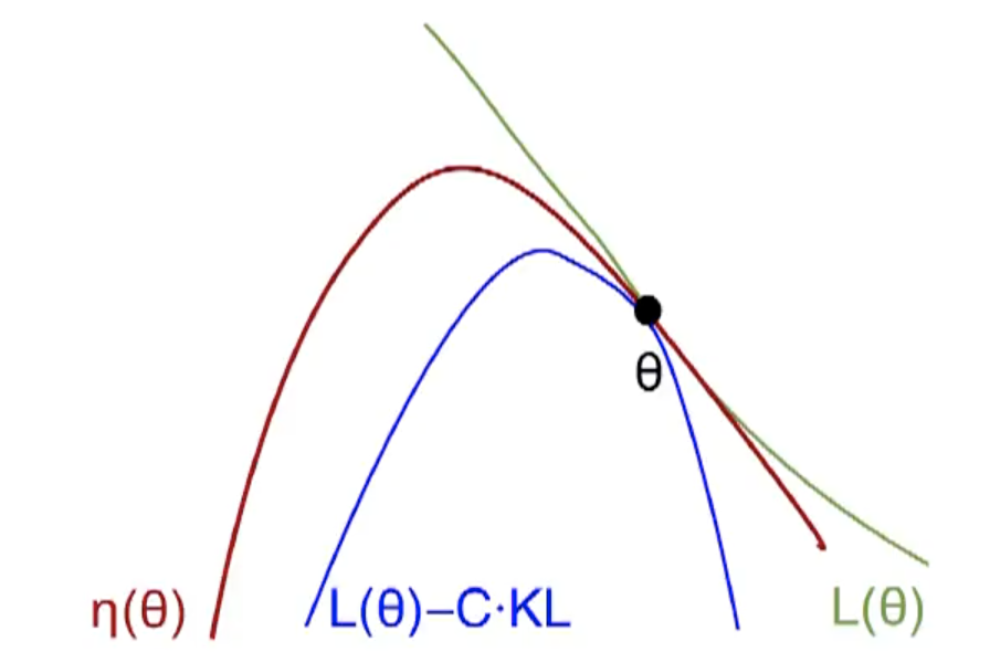
利用不等式:$\eta(\tilde{\pi}) \geq L_{\pi}(\tilde{\pi})-C D_{\mathrm{KL}}^{\max }(\pi, \tilde{\pi})$, where $C=\frac{4 \epsilon \gamma}{(1-\gamma)^{2}}$.
该不等式给出了$\eta(\tilde\pi)$的lower bound $M_i(\pi) = L_{\pi_i}(\pi) - CD_{KL}^{\max}(\pi_i, \pi)$
证明策略的单调性:
$\eta\left(\pi_{i+1}\right) \geqslant M_{i}\left(\pi_{i+1}\right)$, 且 $\eta\left(\pi_{i}\right) = M_{i}\left(\pi_{i}\right)$, 则 $\eta\left(\pi_{i+1}\right)-\eta\left(\pi_{i}\right) \geqslant M_{i}\left(\pi_{i+1}\right)-M\left(\pi_{i}\right)$.
如果新策略能够使得$M_i$最大,我们可以得到$M_i(\pi_{i+1}) - M(\pi_i) \geq 0$, 则 $\eta(\pi_{i+1})-\eta(\pi_i) \geq 0$.
使得$M_i$最大的策略 $\iff$ $\underset{\theta}{\operatorname{maximize}}\left[L_{\theta_{\text {old }}}(\theta)-C D_{\mathrm{KL}}^{\max }\left(\theta_{\text {old }}, \theta\right)\right]$
利用惩罚因子$C$, the step size will be small. –> add constraint on the KL divergence (trust region constraint):
$$
\begin{array}{l}
\underset{\theta}{\operatorname{maximize}} \quad \mathbb{E}{s \sim \rho{\theta_{\text {old}}}, a \sim \pi_{\theta_{old}}}\left[\frac{\pi_{\theta}(a \mid s)}{\pi_{\theta_{old}}(a \mid s)} A_{\theta_{\text {old}}}(s, a)\right] \
\text {subject to} \quad D^{\max}{\mathrm{KL}}\left(\theta{\text {old}}, {\theta}\right) \leq \delta
\end{array}
$$
在约束条件中,利用平均KL散度代替最大KL散度。该问题化简为
$$
\begin{array}{l}
\underset{\theta}{\operatorname{maximize}} \quad \mathbb{E}{s \sim \rho{\theta_{\text {old }}}, a \sim q}\left[\frac{\pi_{\theta}(a \mid s)}{q(a \mid s)} Q_{\theta_{\text {old }}}(s, a)\right] \
\text { subject to} \quad \mathbb{E}{s \sim \rho{\theta_{\text {old}}}}\left[D_{\mathrm{KL}}\left(\pi_{\theta_{\text {old}}}(\cdot \mid s) | \pi_{\theta}(\cdot \mid s)\right)\right] \leq \delta
\end{array}
$$
The objective function (surrogate advantage) is a measure of how policy $\pi_\theta$ performs relative to the old policy $\pi_{\theta_{old}}$ using data from the old policy.
接下来就是利用采样得到数据,然后求样本均值,解决优化问题即可。至此,TRPO理论算法完成。
求解优化问题:
The objective and constraint are both zero when $\theta=\theta_{old}$. Furthermore, the gradient of the constraint with respect to $\theta$ is zero when $\theta=\theta_{old}$. TRPO makes some approximations to get an answer quickly. We Taylor expand the objective and constraint to leading order around $\theta_{old}$:
$$
\begin{array}{c}
\mathcal{L}\left(\theta_{k}, \theta\right) \approx g^{T}\left(\theta-\theta_{k}\right) \
\bar{D}{K L}\left(\theta | \theta{k}\right) \approx \frac{1}{2}\left(\theta-\theta_{k}\right)^{T} H\left(\theta-\theta_{k}\right)
\end{array}
$$
resulting in an approximate optimization problem,
$$
\begin{array}{r}
\theta_{k+1}=\arg \max {\theta} g^{T}\left(\theta-\theta{k}\right) \
\text { s.t. } \frac{1}{2}\left(\theta-\theta_{k}\right)^{T} H\left(\theta-\theta_{k}\right) \leq \delta
\end{array}
$$
This approximate problem can be analytically solved by the methods of Lagrangian duality, yielding the solution:
$$
\theta_{k+1}=\theta_{k}+\sqrt{\frac{2 \delta}{g^{T} H^{-1} g}} H^{-1} g
$$
A problem is that, due to the approximation errors introduced by the Taylor expansion, this may not satisfy the KL constraint, or actually improve the surrogate advantage. TRPO adds a modification to this update rule: a backtracking line search,
$$
\theta_{k+1}=\theta_{k}+\alpha^{j} \sqrt{\frac{2 \delta}{g^{T} H^{-1} g}} H^{-1} g
$$
where $\alpha\in (0,1)$ is the backtracking coefficient, and $j$ is the smallest nonnegative integer such that $\pi_\theta$ satisfies the KL constraint and produces a positive surrogate advantage.
Lastly: computing and storing the matrix inverse, $H^{-1}$, is painfully expensive when dealing with neural network policies with thousands or millions of parameters. TRPO sidesteps the issue by using the conjugate gradient algorithm to solve $Hx=g$ for $x=H^{-1}g$ , requiring only a function which can compute the matrix-vector product $Hx$ instead of computing and storing the whole matrix $H$ directly. This is not too hard to do: we set up a symbolic operation to calculate
$$
H x=\nabla_{\theta}\left(\left(\nabla_{\theta} \bar{D}{K L}\left(\theta | \theta{k}\right)\right)^{T} x\right)
$$
which gives us the correct output without computing the whole matrix.
Over the course of training, the policy typically becomes progressively less random, as the update rule encourages it to exploit rewards that it has already found. This may cause the policy to get trapped in local optima.
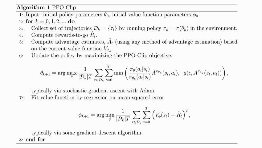
PPO
Fundamental Knowledge:
TRPO:
$$
\begin{array}{ll}
\underset{\theta}{\operatorname{maximize}} & \hat{\mathbb{E}}{t}\left[\frac{\pi{\theta}\left(a_{t} \mid s_{t}\right)}{\pi_{\theta_{\text {old }}}\left(a_{t} \mid s_{t}\right)} \hat{A}{t}\right] \
\text { subject to } & \widehat{\mathbb{E}}{t}\left[\operatorname{KL}\left[\pi_{\theta_{\text {old }}}\left(\cdot \mid s_{t}\right), \pi_{\theta}\left(\cdot \mid s_{t}\right)\right]\right] \leq \delta
\end{array}
$$
This problem can efficiently be approximately solved using the conjugate gradient algorithm, after making a linear approximation to the objective and a quadratic approximation to the constraint. The theory justifying TRPO actually suggests using a penalty instead of a constraint, i.e., solving the unconstrained optimization problem
$$
\underset{\theta}{\operatorname{maximize}} \hat{\mathbb{E}}{t}\left[\frac{\pi{\theta}\left(a_{t} \mid s_{t}\right)}{\pi_{\theta_{\text {old }}}\left(a_{t} \mid s_{t}\right)} \hat{A}{t}-\beta \operatorname{KL}\left[\pi{\theta_{\text {old }}}\left(\cdot \mid s_{t}\right), \pi_{\theta}\left(\cdot \mid s_{t}\right)\right]\right]
$$for some coefficient $\beta$.
a certain surrogate objective (which computes the max KL over states instead of the mean) forms a lower bound (i.e., a pessimistic bound) on the performance of the policy $\pi$.
TRPO uses a hard constraint rather than a penalty because it is hard to choose a single value of $\beta$ that performs well across different problems—or even within a single problem, where the the characteristics change over the course of learning.
Actor-critic:
sensitive to perturbations (small change in parameters of network –> big change of policy space)
In order to address this issue, PPO:
- limits update to policy network, and
- base the update on the ratio of new policy to old. (make the ratio be confined into a range –> not take big step in parameter space)
- Need to account for goodness of state (advantage)
- clip the loss function and take lower bound with minimum function
- Track a fixed length trajectory of memories (instead of many transitions)
- Use multiple network updates per data sample. Use minibatch stochastic gradient ascent
- can use multiple parallel CPU
Important Components:
Update Actor is different
$$
L^{CPI}(\theta) = \hat{\mathbb E} \left[ \frac{\pi_\theta(a_t|s_t)}{\pi_{\theta_{old}}(a_t|s_t) }\hat A_t \right] = \hat{\mathbb E} \left[r_t(\theta) \hat A_t \right]
$$- based on ratio of new policy to old policy (can use log)
- consider the advantage
Only maximize $L^{CPI}(\theta)$ will lead to large policy update, –> Modify objective
Adding epsilon (about 0.2) for clip/min operations
$$
L^{CPI}(\theta) = \hat{\mathbb E} \left[ \min\left(r_t(\theta)\hat{A}_t;, ; \operatorname{clip}(r_t(\theta), 1-\epsilon, 1+\epsilon) \right)\hat{A}_t \right]
$$pessimistic lower bound to the loss
- smaller loss, smaller gradient, smaller update
Advantages at each time step:
$$
\hat{A}t = \delta_t + (\gamma\lambda)\delta{t+1} + \cdots +(\gamma\lambda)^{T-t+1}\delta_{T-1}
$$
where $\delta_t = r_t + \gamma V(s_{t+1}) - V(s_t)$.- show the benefit of the new state over the old state
- $\lambda$ is a smoothing parameter (about 0.95) to help to reduce variance
- Nested for loops
Critic loss is straightforward
- Return = advantage + critic_value (from memory)
- $L_{critic}$ = MSE( return - critic_value ) [from network]
Total loss is sum of clipped actor and critic
$$
L_t^{CLIP+VF+S} = \hat{\mathbb E} \left[ L_t^{CLIP}(\theta) - c_1 L_t^{VF} + c_2 S\pi_\theta \right]
$$- coefficient $c_1$ of the critic
- $S$ term is the entropy term [which is required if the actor and critic are coupled].
总结:
PPO: off-policy
通过importance sampling实现离线更新策略(可以使用行为策略所得到的数据用来更新目标策略)
使用$\theta_{old}$采样的数据,训练$\theta$这个actor,过程中$\theta_{old}$是fixed的所以可以重复使用用$\theta_{old}$的数据训练$\theta$许多次,增加数据利用率,提高训练速度。也就是说,在importance sampling中,我们使用$\theta_{old}$获得数据,来估计$\theta$的期望分布。、
但是注意,此时两种策略的分布不能差别很大。–> 引入了约束条件。
- TRPO是加入了KL($\theta_{old},\theta$) divergence的constraint
- PPO是在目标函数后加入了关于$\beta$KL($\theta_{old},\theta$)的惩罚项.
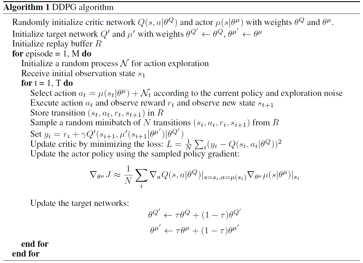
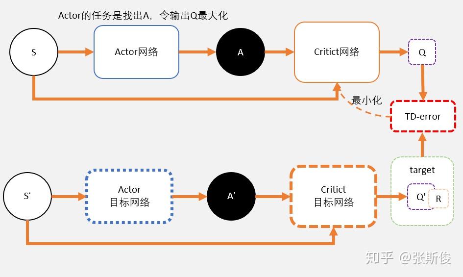
DDPG
同样,也是Actor-Critic架构。
Actor:
- Input: state $s$
- Output: action $a$。 【在Actor-Critic方法中,输出的是一个概率分布】
- 更新方法是基于梯度上升的。
- 该网络的损失函数就是从critic网络中获取的Q值的平均值,在实现的过程中,需要加入负号,即最小化损失函数,来与深度学习框架保持一致。用数学公式表示其损失函数就是:$L_{actor}=\mathbb E \left[{Q(s,a|\theta^Q)}|_{s=s_t,a=\mu(s_t|\theta^\mu)} \right]$.
Critic:
- Input: state $s$ and action $a$
- Output: Q value $Q(s,a)$。 【在Actor-Critic方法中,输出的是$V(s)$】
- 通过最小化目标网络与现有网络之间的均方误差来更新现有网络的参数,
加入experience replay buffer,存储agent与env之间的交互数据。
在实际操作中,如果更新目标在变化,会导致更新困难。–> use “soft” target updates, rather than directly copy the weights –> 方法:添加target actor 和 target critic 网络。并在更新target 网络参数时增加权重$\tau$,即每一步仅采用相对小的权重采用相应训练中的network更新;如此的目的在于尽可能保障训练能够收敛;
Exploration via random process, 为actor采取的action基础上增加一定的随机扰动, 以保障一定的探索完整动作空间的几率。一般的, 相应随机扰动的幅度随着训练的深入而逐步递减;
Batch normalization, 为每层神经网络之前加入batch normalization层, 可以降低不对状态量取值范围差异对模型稳定性的影响程度。
TD3
DDPG起源于DQN,是DQN解决连续控制问题的一个解决方法。而DQN有一个众所周知的问题,就是Q值会被高估。这是因为我们用$\operatorname{argmax}Q(s’)$去代替$V(s’)$,去评估$Q(s)$。当我们每一步都这样做的时候,很容易就会出现高估$Q$值的情况。类似地,DDPG也会有这个问题。可以借鉴double DQN的思路来解决这个问题。在TD3中,可以用两套网络估算$Q$值,相对较小的那个作为我们更新的目标。这就是TD3的基本思路。
DDPG算法涉及了4个网络,TD3需要用到6个网络。

Actor:
与DDPG相同
Critic:
- 两个target ciritc网络,用于计算两个Q值:$Q_1(A’)$和$Q_2(A’)$.
- $\min(Q_1(A’), Q_2(A’))$用来计算target value,i.e. $y_i = r+ \gamma \min(Q_1(A’), Q_2(A’))$. 而计算出的target value也是两个critic网络的更新目标。
- 两个critic 网络的意义:虽然更新目标一样,两个网络会越来越趋近与和实际q值相同。但由于网络参数的初始值不一样,会导致计算出来的值有所不同。所以我们可以选择较小的值去估算q值,避免q值被高估。
送
SAC
Maximum Entropy RL
之前的RL算法中,学习目标主要是学习一个policy使得累积reward的期望值最大:$\pi^{*}=\arg \max {\pi} \mathbb{E}{\left(s_{t}, a_{t}\right) \sim \rho_{\pi}}\left[\sum_{t} R\left(s_{t}, a_{t}\right)\right]$.
而最大熵RL的学习目标,除了学习一个policy使得累积reward最大,还要求policy的每一次输出的action的entropy最大:
$$
\pi^{*}=\arg \max {\pi} \mathbb{E}{\left(s_{t}, a_{t}\right) \sim \rho_{\pi}} \left[\sum_{t} \underbrace{R\left(s_{t}, a_{t}\right)}{\text {reward }}+\alpha \underbrace{H\left(\pi\left(\cdot \mid s{t}\right)\right)}_{\text {entropy }}\right]
$$
$\alpha$是temperature parameter决定entropy项和reward之间的relative importance。通过增加entropy项,可使得策略随机化,即输出的每一个action的概率尽可能均匀,而不是集中在一个action上。从而鼓励exploration,也可以学到更多near-optimal行为(也就是在一些状态下, 可能存在多个action都是最优的,那么使得选择它们的概率相同,可以提高学习速度)。
在信息论中,熵(entropy)是接收的每条消息中包含的信息的平均量,又被稱為信息熵、信源熵、平均自信息量。这里,“消息”代表来自分布或数据流中的事件、样本或特征。(熵最好理解为不确定性的量度而不是确定性的量度,因为越随机的信源的熵越大。)来自信源的另一个特征是样本的概率分布。这里的想法是,比较不可能发生的事情,当它发生了,会提供更多的信息。由于一些其他的原因,把信息(熵)定义为概率分布的对数的相反数是有道理的。事件的概率分布和每个事件的信息量构成了一个随机变量,这个随机变量的均值(即期望)就是这个分布产生的信息量的平均值(即熵)。
Soft Policy Iteration
Soft policy evaluation
思路1(通过DP得到Soft bellman equation):
- 因此可以得到Soft Bellman Backup equation (Entropy项额外乘上$\alpha$系数) :
$$
q_{\pi}(s, a)=r(s, a)+\gamma \sum_{s^{\prime} \in \mathcal{S}} \mathcal{P}{s s^{\prime}}^{a} \sum{a^{\prime} \in \mathcal{A}} \pi\left(a^{\prime} \mid s^{\prime}\right)\left(q_{\pi}\left(s^{\prime}, a^{\prime}\right)-\alpha \log \left(\pi\left(a^{\prime} \mid s^{\prime}\right)\right)\right.
$$
可以得到Soft Bellman Backup的 更新公式:
$$
Q_{\text{soft}}\left(s_{t}, a_{t}\right)=r\left(s_{t}, a_{t}\right)+\gamma \mathbb{E}{s{t+1}, a_{t+1}}\left[Q_{\text{soft}}\left(s_{t+1}, a_{t+1}\right)-\alpha \log \left(\pi\left(a_{t+1} \mid s_{t+1}\right)\right)\right]
$$
思路2(将entropy嵌入reward):
- Reward with entropy:
$$
r_{\text{soft}}\left(s_{t}, a_{t}\right)=r\left(s_{t}, a_{t}\right)+\gamma \alpha \mathbb{E}{s{t+1} \sim \rho} H\left(\pi\left(\cdot \mid s_{t+1}\right)\right)
$$
将该reward代入Bellman equation $Q\left(s_{t}, a_{t}\right)=r\left(s_{t}, a_{t}\right)+\gamma \mathbb{E}{s{t+1}, a_{t+1}}\left[Q\left(s_{t+1}, a_{t+1}\right)\right]$, 得到
$$
\begin{array}{rCl}
Q_{\text{soft}}\left(s_{t}, a_{t}\right) &=& r\left(s_{t}, a_{t}\right)+ \gamma \alpha \mathbb{E}{s{t+1} \sim \rho} H\left(\pi\left(\cdot \mid s_{t+1}\right)\right) + \gamma \mathbb{E}{s{t+1}, a_{t+1}}\left[Q_{\text{soft}}\left(s_{t+1}, a_{t+1}\right)\right] \
&=& r\left(s_{t}, a_{t}\right)+ \gamma \mathbb{E}{s{t+1}\sim\rho,a_{t+1}\sim\pi} \left[Q_{\text{soft}}\left(s_{t+1}, a_{t+1}\right)\right] + \gamma \alpha \mathbb{E}{s{t+1}\sim\rho} H\left(\pi\left(\cdot \mid s_{t+1}\right)\right) \
&=& r\left(s_{t}, a_{t}\right)+ \gamma \mathbb{E}{s{t+1}\sim\rho} \mathbb{E}{a{t+1}\sim\pi} \left[Q_{\text{soft}}\left(s_{t+1}, a_{t+1}\right)\right] - \gamma \alpha \mathbb{E}{s{t+1}\sim\rho}\mathbb{E}{a{t+1}\sim\pi} \log\pi(a_{t+1}|s_{t+1}) \
&=& r\left(s_{t}, a_{t}\right)+ \gamma \mathbb{E}{s{t+1}\sim\rho} \left[ \mathbb{E}{a{t+1}\sim\pi}\left[Q_{\text{soft}}\left(s_{t+1}, a_{t+1}\right) - \alpha \log\pi(a_{t+1}|s_{t+1}) \right]\right] \
&=& r\left(s_{t}, a_{t}\right)+ \gamma \mathbb{E}{s{t+1},a_{t+1}}\left[Q_{\text{soft}}\left(s_{t+1}, a_{t+1}\right) - \alpha \log\pi(a_{t+1}|s_{t+1}) \right] \
\end{array}
$$
该结果也和思路1得到的结果相同。
因此,根据$Q\left(s_{t}, a_{t}\right)=r\left(s_{t}, a_{t}\right)+\gamma \mathbb{E}{s{t+1} \sim \rho}\left[V\left(s_{t+1}\right)\right]$,可得到$V_{\text{soft}}(s_t)$:
$$
V_{\text{soft}}\left(s_{t}\right)=\mathbb{E}{a{t} \sim \pi}\left[Q_{\text {soft}}\left(s_{t}, a_{t}\right)-\alpha \log \pi\left(a_{t} \mid s_{t}\right)\right]
$$
Soft Policy Evaluation: 固定policy,使用soft Bellman equation更新Q value直到收敛
$$
Q_{\text{soft}}\left(s_{t}, a_{t}\right)=r\left(s_{t}, a_{t}\right)+\gamma \mathbb{E}{s{t+1}, a_{t+1}}\left[Q_{\text{soft}}\left(s_{t+1}, a_{t+1}\right)-\alpha \log \left(\pi\left(a_{t+1} \mid s_{t+1}\right)\right)\right]
$$
Soft policy improvement
stochastic policy的重要性:面对多模的(multimodal)的Q function,传统的RL只能收敛到一个选择(左图),而更优的办法是右图,让policy也直接符合Q的分布。
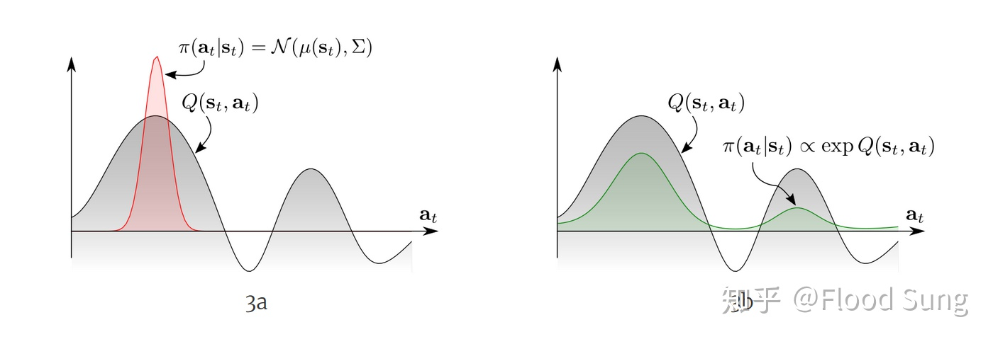
这里,通过定义energy-based policy as:$\pi(a_t|s_t) \propto \exp(-\mathcal E(s_t,a_t))$。设定$\mathcal E(s_t,a_t)=-\frac{1}{\alpha}Q_{\text{soft}}(s_t,a_t)$, 可以得到$\pi(a_t|s_t) \propto \exp(-\mathcal E(s_t,a_t))$。根据$V_{\text{soft}}\left(s_{t}\right)=\mathbb{E}{a{t} \sim \pi}\left[Q_{\text {soft}}\left(s_{t}, a_{t}\right)-\alpha \log \pi\left(a_{t} \mid s_{t}\right)\right]$, 可以得到
$$
\begin{array}{rCl}
\pi(s_t,a_t) &=& \exp \left( \frac{1}{\alpha} \left(Q_{\text{soft}}(s_t,a_t) - V_{\text{soft}}(s_t) \right)\right) \
&=& \frac{\frac{1}{\alpha}Q_{\text{soft}}(s_t,a_t)}{\frac{1}{\alpha}V_{\text{soft}}(s_t)} \propto Q_{\text{soft}}(s_t,a_t)
\end{array}
$$
其中,$\exp \left(\frac{1}{\alpha} V_{\text {soft }}\left(s_{t}\right)\right)=\int \exp \left(\frac{1}{\alpha} Q_{\text {soft }}\left(s_{t}, a\right)\right) d a$,因此,$V_{\text {soft }}\left(s_{t}\right) \triangleq \alpha \log \int \exp \left(\frac{1}{\alpha} Q_{\text {soft }}\left(s_{t}, a\right)\right) d a$
所以,$\underset{a}{\operatorname{soft max}} f(a):=\log \int \exp f(a) d a$, –> $Q_{\text {soft }}\left(s_{t}, a_{t}\right)=\mathbb{E}\left[r_{t}+\gamma \underset{a}{\operatorname{soft max}} Q\left(s_{t+1}, a\right)\right]$.
因此可以得到:$\pi_{\text{MaxEnt}}^{}\left(a_{t} \mid s_{t}\right)=\exp \left(\frac{1}{\alpha}\left(Q_{\text {soft }}^{}\left(s_{t}, a_{t}\right)-V_{\text {soft}}^{*}\left(s_{t}\right)\right)\right)$。
Soft Policy Improvement: 更新policy towards the exponential of new Q-function. Restrict the policy to some set of policies, like Gaussian.
$$
\pi^{\prime}=\arg \min {\pi{k} \in \Pi} D_{K L}\left(\pi_{k}\left(\cdot \mid s_{t}\right) \Big| \frac{\exp \left(\frac{1}{\alpha} Q_{\text {soft }}^{\pi}\left(s_{t}, \cdot\right)\right)}{Z_{\text {soft }}^{\pi}\left(s_{t}\right)}\right)
$$
其中, $Z^\pi_{\text{soft}}(s_t)$ 就是是一个配分函数,用于归一化分布,在求导的时候可以直接忽略。此处,通过KL divergence来趋近$\exp(Q_{\text{soft}}^{\pi}(s_t,\cdot))$ ,从而限制policy在一定范围的policies $\Pi$中,从而变得tractable,policy的分布可以是高斯分布。
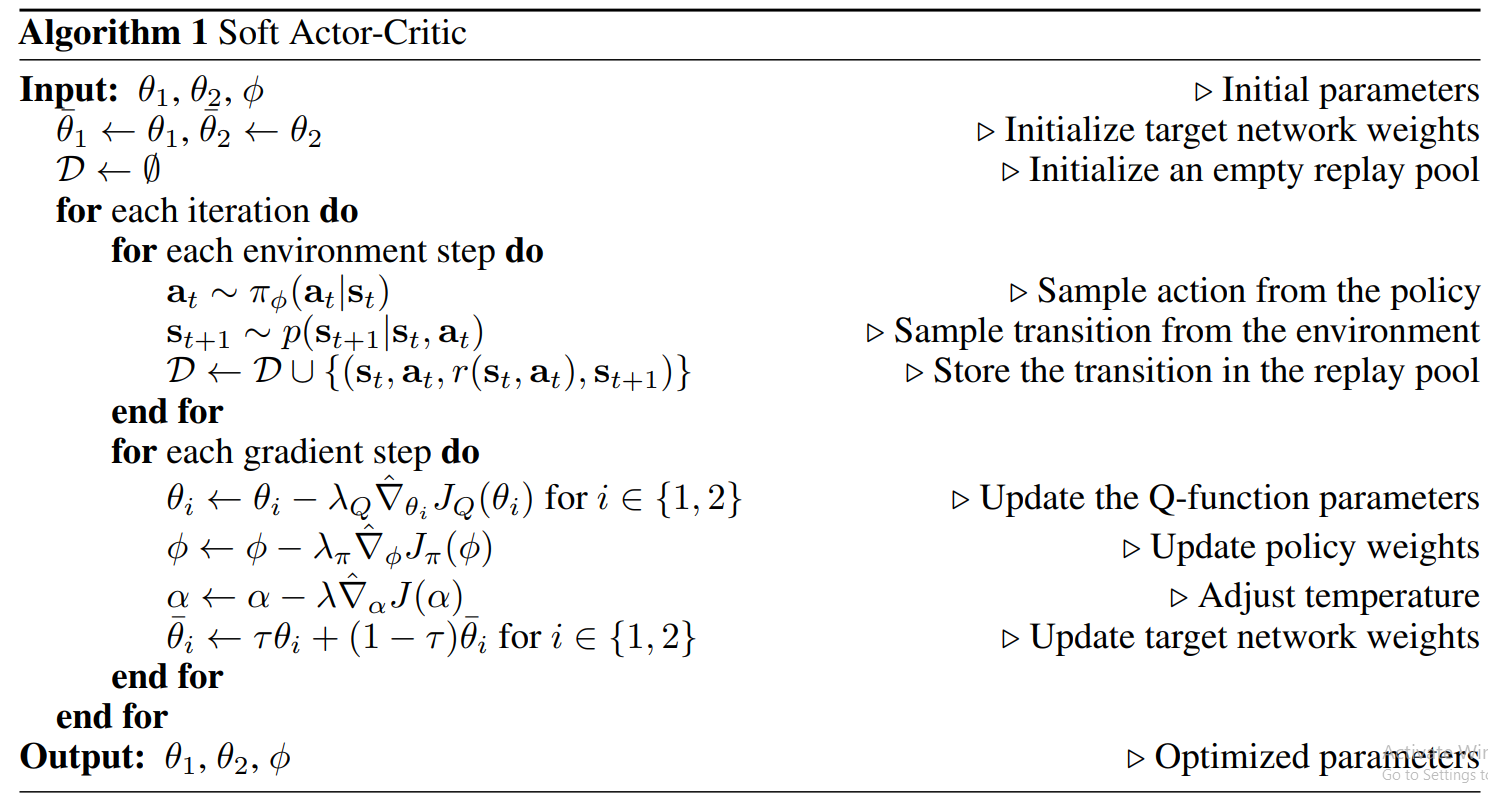
Soft Actor Critic
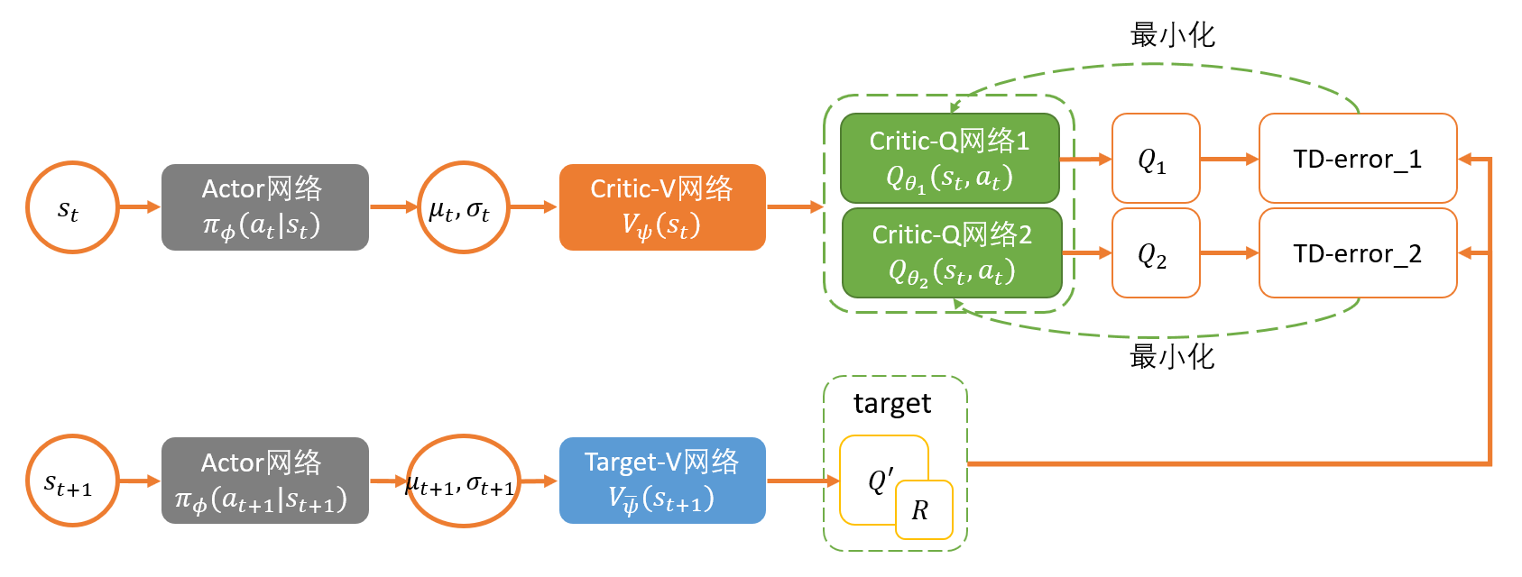
旧版SAC:
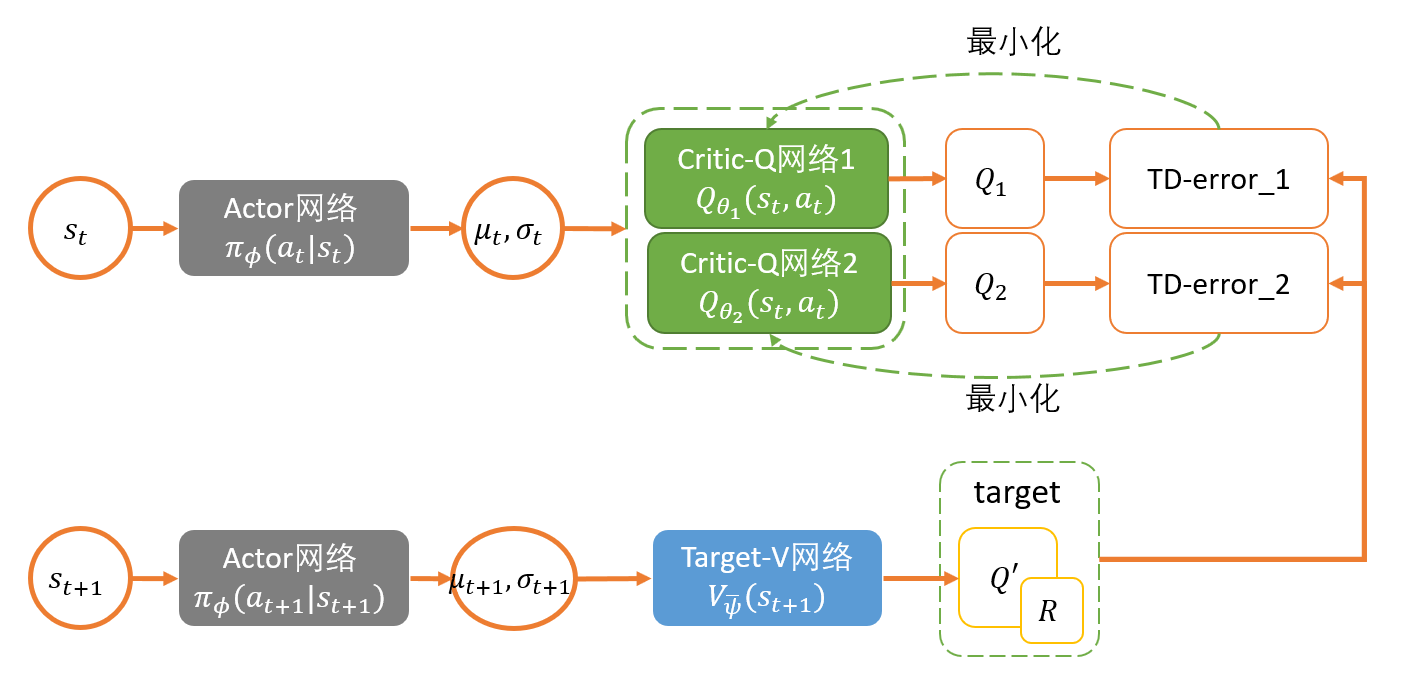
新版SAC:
Critic:
$$
\begin{aligned}
J_{Q}(\theta) &=\mathbb{E}{\left(s{t}, a_{t}, s_{t+1}\right) \sim \mathcal{D}}\left[\frac{1}{2}\left(Q_{\theta}\left(s_{t}, a_{t}\right)-\left(r\left(s_{t}, a_{t}\right)+\gamma V_{\bar{\theta}}\left(s_{t+1}\right)\right)\right)^{2}\right] \
&=\mathbb{E}{\left(s{t}, a_{t}, s_{t+1}\right) \sim \mathcal{D}, a_{t+1} \sim \pi_{\phi}}\left[\frac{1}{2}\left(Q_{\theta}\left(s_{t}, a_{t}\right)-\left(r\left(s_{t}, a_{t}\right)+\gamma\left(Q_{\bar{\theta}}\left(s_{t+1}, a_{t+1}\right)-\alpha \log \left(\pi_{\phi}\left(a_{t+1} \mid s_{t+1}\right)\right)\right)\right)\right)^{2}\right]
\end{aligned}
$$
这里和DDPG一样,构造了一个target soft Q 网络带参数$\bar \theta$,这个参数通过exponentially moving average Q网络的参数$\theta$得到。在第一个版本的SAC中,他们单独定义了Value网络进行更新,
在新版的SAC中,由于自动更新temperature $\alpha$就直接使用Q网络更新。
Actor:
$$
\begin{aligned}
J_{\pi}(\phi) &=D_{\mathrm{KL}}\left(\pi_{\phi}\left(. \mid s_{t}\right) | \exp \left(\frac{1}{\alpha} Q_{\theta}\left(s_{t}, .\right)-\log Z\left(s_{t}\right)\right)\right) \
&=\mathbb{E}{s{t} \sim \mathcal{D}, a_{t} \sim \pi_{\phi}}\left[\log \left(\frac{\pi_{\phi}\left(a_{t} \mid s_{t}\right)}{\exp \left(\frac{1}{\alpha} Q_{\theta}\left(s_{t}, a_{t}\right)-\log Z\left(s_{t}\right)\right)}\right)\right] \
&=\mathbb{E}{s{t} \sim \mathcal{D}, a_{t} \sim \pi_{\phi}}\left[\log \pi_{\phi}\left(a_{t} \mid s_{t}\right)-\frac{1}{\alpha} Q_{\theta}\left(s_{t}, a_{t}\right)+\log Z\left(s_{t}\right)\right]
\end{aligned}
$$
这里的action我们采用reparameterization trick来得到,即 $a_{t}=f_{\phi}\left(\varepsilon_{t} ; s_{t}\right)=f_{\phi}^{\mu}\left(s_{t}\right)+\varepsilon_{t} \odot f_{\phi}^{\sigma}\left(s_{t}\right)$。$f$函数输出平均值和方差,然后$\epsilon$是noise,从标准正态分布采样。使用这个trick,整个过程就是完全可微的(loss 乘以$\alpha$并去掉不影响梯度的常量log partition function $Z(s_t)$:
$$
J_{\pi}(\phi)=\mathbb{E}{s{t} \sim \mathcal{D}, \varepsilon \sim \mathcal{N}}\left[\alpha \log \pi_{\phi}\left(f_{\phi}\left(\varepsilon_{t} ; s_{t}\right) \mid s_{t}\right)-Q_{\theta}\left(s_{t}, f_{\phi}\left(\varepsilon_{t} ; s_{t}\right)\right)\right]
$$Update temperature
前面的SAC中,我们只是人为给定一个固定的temperature $\alpha$ 作为entropy的权重,但实际上由于reward的不断变化,采用固定的temperature并不合理,会让整个训练不稳定,因此,有必要能够自动调节这个temperature。当policy探索到新的区域时,最优的action还不清楚,应该调高temperature 去探索更多的空间。当某一个区域已经探索得差不多,最优的action基本确定了,那么这个temperature就可以减小。
这里,SAC的作者构造了一个带约束的优化问题,让平均的entropy权重是有限制的,但是在不同的state下entropy的权重是可变的,即 $\max {\pi{0}, \ldots, \pi_{T}} \mathbb{E}\left[\sum_{t=0}^{T} r\left(s_{t}, a_{t}\right)\right]$ s.t. $\forall t, \mathcal{H}\left(\pi_{t}\right) \geq \mathcal{H}_{0}$
最后得到temperature的loss:
$$
J(\alpha)=\mathbb{E}{a{t} \sim \pi_{t}}\left[-\alpha \log \pi_{t}\left(a_{t} \mid \pi_{t}\right)-\alpha \mathcal{H}_{0}\right]
$$
DDPG与SAC的区别:
DDPG训练得到的是一个deterministic policy确定性策略,也就是说这个策略对于一种状态state只考虑一个最优的动作。Deterministic policy的最终目标找到最优路径。
Stochastic policy随机策略在实际应用中往往是更好的做法。比如我们让机器人抓取一个水杯,机器人是有无数条路径去实现这个过程的,而并不是只有唯一的一种做法。因此,我们就需要DRL算法能够给出一个随机策略,在每一个state上都能输出每一种action的概率,比如有3个action都是最优的,概率一样都最大,那么我们就可以从这些action中随机选择一个做出action输出。最大熵maximum entropy的核心思想就是不遗落到任意一个有用的action,有用的trajectory。对比DDPG的deterministic policy的做法,看到一个好的就捡起来,差一点的就不要了,而最大熵是都要捡起来,都要考虑。
Stochastic policy要求熵最大,就意味着神经网络需要去explore探索所有可能的最优路径,优势如下:
- 学到policy可以作为更复杂具体任务的初始化。因为通过最大熵,policy不仅仅学到一种解决任务的方法,而是所有all。因此这样的policy就更有利于去学习新的任务。比如我们一开始是学走,然后之后要学朝某一个特定方向走。
- 更强的exploration能力,这是显而易见的,能够更容易的在多模态reward (multimodal reward)下找到更好的模式。比如既要求机器人走的好,又要求机器人节约能源
- 更robust鲁棒,更强的generalization。因为要从不同的方式来探索各种最优的可能性,也因此面对干扰的时候能够更容易做出调整。(干扰会是学习过程中看到的一种state,既然已经探索到了,学到了就可以更好的做出反应,继续获取高reward)
基于最大熵的RL算法有什么优势?
以前用deterministic policy的算法,我们找到了一条最优路径,学习过程也就结束了。现在,我们还要求熵最大,就意味着神经网络需要去explore探索所有可能的最优路径,这可以产生以下多种优势:
1)学到policy可以作为更复杂具体任务的初始化。因为通过最大熵,policy不仅仅学到一种解决任务的方法,而是所有all。因此这样的policy就更有利于去学习新的任务。比如我们一开始是学走,然后之后要学朝某一个特定方向走。
2)更强的exploration能力,这是显而易见的,能够更容易的在多模态reward (multimodal reward)下找到更好的模式。比如既要求机器人走的好,又要求机器人节约能源
3)更robust鲁棒,更强的generalization。因为要从不同的方式来探索各种最优的可能性,也因此面对干扰的时候能够更容易做出调整。(干扰会是神经网络学习过程中看到的一种state,既然已经探索到了,学到了就可以更好的做出反应,继续获取高reward)
Summary
DRL中,特别是面向连续控制continuous control,主要的三类算法:
- TRPO,PPO
- DDPG及其拓展(D4PG,TD3等)
- Soft Q-Learning, Soft Actor-Critic
PPO算法是目前最主流的DRL算法,同时面向离散控制(discrete control)和连续控制(continuous control)。但是PPO是一种on-policy的算法,面临着严重的sample inefficiency,需要巨量的采样才能学习,因此在实际应用中较难实现。
DDPG及其拓展则是面向连续控制的off policy算法,相对PPO 更sample efficient。DDPG训练的是一种确定性策略deterministic policy,即每一个state下都只考虑最优的一个动作。
Soft Actor-Critic (SAC)是面向Maximum Entropy Reinforcement learning 开发的一种off policy算法,和DDPG相比,Soft Actor-Critic使用的是随机策略stochastic policy,相比确定性策略具有一定的优势。Soft Actor-Critic效果好,且能直接应用到真实机器人上。